Principal Components Analysis ( PCA)

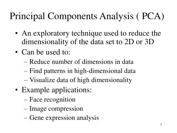
1. Principal Components Analysis ( PCA) • An exploratory technique used to reduce the dimensionality of the data set to 2D or 3D • Can be used to: • Reduce number of dimensions in data • Find patterns in high-dimensional data • Visualize data of high dimensionality • Example applications: • Face recognition • Image compression • Gene expression analysis

2. Principal Components Analysis Ideas ( PCA) • Does the data set ‘span’ the whole of d dimensional space? • For a matrix of m samples x n genes, create a new covariance matrix of size n x n. • Transform some large number of variables into a smaller number of uncorrelated variables called principal components (PCs). • developed to capture as much of the variation in data as possible

3. Y1 Y2 x x x x x x x x x x x x x x x x x x x x x x x x x • Principal Component Analysis • See online tutorials such as http://www.cs.otago.ac.nz/cosc453/student_tutorials/principal_components.pdf X2 Note: Y1 is the first eigen vector, Y2 is the second. Y2 ignorable. X1 Key observation: variance = largest!

4. Principal Component Analysis: one attribute first • Question: how much spread is in the data along the axis? (distance to the mean) • Variance=Standard deviation^2

5. Now consider two dimensions • Covariance: measures thecorrelation between X and Y • cov(X,Y)=0: independent • Cov(X,Y)>0: move same dir • Cov(X,Y)<0: move oppo dir

6. More than two attributes: covariance matrix • Contains covariance values between all possible dimensions (=attributes): • Example for three attributes (x,y,z):

7. Eigenvalues & eigenvectors • Vectors x having same direction as Ax are called eigenvectors of A (A is an n by n matrix). • In the equation Ax=x,  is called an eigenvalue of A.

8. Eigenvalues & eigenvectors • Ax=x  (A-I)x=0 • How to calculate x and : • Calculate det(A-I), yields a polynomial (degree n) • Determine roots to det(A-I)=0, roots are eigenvalues  • Solve (A- I) x=0 for each  to obtain eigenvectors x

9. Principal components • 1. principal component (PC1) • The eigenvalue with the largest absolute value will indicate that the data have the largest variance along its eigenvector, the direction along which there is greatest variation • 2. principal component (PC2) • the direction with maximum variation left in data, orthogonal to the 1. PC • In general, only few directions manage to capture most of the variability in the data.

10. Let be the mean vector (taking the mean of all rows) Adjust the original data by the mean X’ = X – Compute the covariance matrix C of adjusted X Find the eigenvectors and eigenvalues of C. For matrix C, vectors e (=column vector) having same direction as Ce : eigenvectors of C is e such thatCe=e,  is called an eigenvalue of C. Ce=e  (C-I)e=0 Most data mining packages do this for you. Steps of PCA

11. Eigenvalues • Calculate eigenvalues  and eigenvectors x for covariance matrix: • Eigenvalues j are used for calculation of [% of total variance] (Vj) for each component j:

12. Principal components - Variance

13. Transformed Data • Eigenvalues j corresponds to variance on each component j • Thus, sort by j • Take the first p eigenvectors ei; where p is the number of top eigenvalues • These are the directions with the largest variances

14. An Example Mean1=24.1 Mean2=53.8

15. Covariance Matrix • C= • Using MATLAB, we find out: • Eigenvectors: • e1=(-0.98,-0.21), 1=51.8 • e2=(0.21,-0.98), 2=560.2 • Thus the second eigenvector is more important!

16. If we only keep one dimension: e2 • We keep the dimension of e2=(0.21,-0.98) • We can obtain the final data as

20. PCA –> Original Data • Retrieving old data (e.g. in data compression) • RetrievedRowData=(RowFeatureVectorT x FinalData)+OriginalMean • Yields original data using the chosen components

21. Principal components • General about principal components • summary variables • linear combinations of the original variables • uncorrelated with each other • capture as much of the original variance as possible

22. Applications – Gene expression analysis • Reference: Raychaudhuri et al. (2000) • Purpose: Determine core set of conditions for useful gene comparison • Dimensions: conditions, observations: genes • Yeast sporulation dataset (7 conditions, 6118 genes) • Result: Two components capture most of variability (90%) • Issues: uneven data intervals, data dependencies • PCA is common prior to clustering • Crisp clustering questioned : genes may correlate with multiple clusters • Alternative: determination of gene’s closest neighbours

23. Two Way (Angle) Data Analysis Conditions 101–102 Genes 103–104 Genes 103-104 Gene expression matrix Gene expression matrix Samples 101-102 Sample space analysis Gene space analysis

24. PCA - example

25. PCA on all GenesLeukemia data, precursor B and T Plot of 34 patients, dimension of 8973 genes reduced to 2

26. PCA on 100 top significant genes Leukemia data, precursor B and T Plot of 34 patients, dimension of 100 genes reduced to 2

27. PCA of genes (Leukemia data) Plot of 8973 genes, dimension of 34 patientsreduced to 2