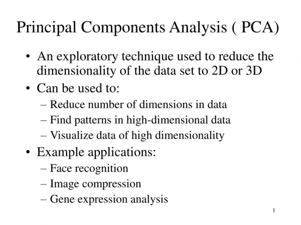
Principal Components Analysis
Principal Components Analysis. BMTRY 726 3/27/14. Uses. Goal : Explain the variability of a set of variables using a “small” set of linear combinations of those variables Why : There are several reasons we may want to do this (1) Dimension Reduction (use k of p components)

Principal Components Analysis
E N D
Presentation Transcript
Principal Components Analysis BMTRY 726 3/27/14
Uses Goal: Explain the variability of a set of variables using a “small” set of linear combinations of those variables Why: There are several reasons we may want to do this (1) Dimension Reduction (use k of p components) -Note, total variability still requires p components (2) Identify “hidden” underlying relationships (i.e. patterns in the data) -Use these relationships in further analyses (3) Select subsets of variables
“Exact” Principal Components We can represent data X as linear combinations of p random measurements on j = 1,2,…,nsubjects
“Exact” Principal Components Principal components are those combinations that are: (1) Uncorrelated (linear combinations Y1, Y2,…, Yp) (2) Variance as large as possible (3) Subject to:
Finding PC’s Under Constraints • So how do we find PC’s that meet the constraints we just discussed? • We want to maximize subject to the constraint that • This constrained maximization problem can be done using the method of Lagrange multipliers • Thus we want to maximize the function
Finding PC’s Under Constraints • Differentiate w.r.t ai:
Finding PC’s Under Constraints • But how do we choose our eigenvector (i.e. which eigenvector corresponds to which PC?) • We can see that what we want to maximize is • So we choose li to be as large as possible • If l1 is our largest eigenvalue with corresponding eigenvector ei then the solution for our max is
Finding PC’s Under Constraints • Recall we had a second constraint • We could conduct a second Lagrangian maximization to find our second PC • However we already know that eigenvectors are independent (so this constraint is met) • We choose the order of the PCs by the magnitude of the eigenvalues
“Exact” Principal Components So we can compute the PCs from the variance matrix of X, S:
Properties We can also find the moments of our PC’s
Properties We can also find the moments of our PC’s
Properties Normality assumption not required to find PC’s If Xj ~ Np(m,S) then: Total Variance:
Principal Components Consider data with p random measures on j = 1,2,…,nsubjects For the jth subject we then have the random vector X2 m2 X1 m1
Graphic Representation X2 Now suppose X1, X2 ~ N2(m, S) Y1axis selected to maximize variation in the scores Y2axis must be orthogonal to Y1 and maximize variation in the scores Y1 Y2 X1
Dimension Reduction Proportion of total variance accounted for by the first k components is If the proportion of variance accounted for by the first k principal components is large, we might want to restrict our attention to only these first k components Keep in mind, components are simply linear combinations of the original p measurements Ideally look for meaningful interpretations of our choose kcomponents
PC’s from Standardized Variables We may want to standardize our variables before finding PCs
PC’s from Standardized Variables So the covariance of V equals the correlation of X We can define our PC’s for Z the same way as before….
Estimation In general we do not know what S is- we must estimate if from the sample So what are our estimated principal components?
Sample Properties In general we do not know what S is- estimate it from sample So what are our estimated principal components?
Centering We often center our observations before defining our PCs The centered PCs are found according to:
Example Jolicoeur and Mosimann (1960) conducted a study looking at the relationship between size and shape of painted turtle carapaces. We can develop PC’s for natural log of length, width, and height of female turtles’ carapaces
Example The first PC is: This might be interpreted as an overall size component Shell dimensions large Shell dimensions small Small values y1 Large values y1
Example The second PC is: Emphasizes contrast between length and height of the shell Small values y2 Large values y2
Example The third PC is: Emphasizes contrast between width and length of the shell Small values y3 Large values y3
Example Consider the proportion of variability accounted for by each PC
Example How are the PCs correlated with each of the x’s? Then
Interpretation of PCs Consider data x1, x2, …., xp: PCs are actually projections onto the estimated eigenvectors -1st PC is the one with the largest projection -For data reduction, only use PCA if the eigenvalues vary -If x’s are uncorrelated, we can’t really do data reduction
Choosing Number of PCs Often the goal of PCA is dimension reduction of data Select a limited number of PCs that capture majority of the variability in the data How do we decide how many PCs to include: 1. Scree plot: plot of versus i 2. Select all PCs with (for standardized observations) 3. Choose some proportion of the variance you want to account for
Choosing Number of PCs Should principal components that only account for a small proportion of variance always be ignored? Not necessarily, they may indicate near perfect colinearities among traits In the turtle example, this is true-very little variation of the variation in shell measurements can be attributed to the 2nd and 3rd components
Large Sample Properties If n is large, there are nice properties we can use
Large Sample Properties Also for our estimated eigenvectors These results assume that X1, X2, …., Xnare N(m, S)
Summary Principal component analysis most useful for dimensionality reduction Can also be used for identifying colinear variables Note, use of PCA in a regression setting is therefore one way to handle multi-colinearity A caveat… principal components can be difficult to interpret and should therefore be used with caution

