MODELING OF SUBGRID-SCALE MIXING IN LARGE-EDDY SIMULATION OF SHALLOW CONVECTION

1. MODELING OF SUBGRID-SCALE MIXING IN LARGE-EDDY SIMULATION OF SHALLOW CONVECTION Dorota Jarecka1 Wojciech W. Grabowski2 Hanna Pawlowska1 Sylwester Arabas1 1 Institute of Geophysics, University of Warsaw, Poland 2 National Center for Atmospheric Research, USA

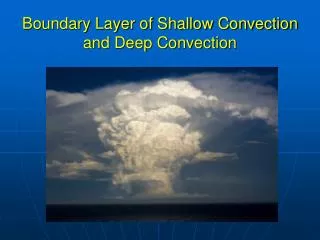
2. Motivation Shallow convective clouds are strongly diluted by entrainment

3. Overview For atmospheric LES models, subgrid-scale mixing should cover wide range of situations: from extremely inhomogeneous at scales close to model gridlength, to homogeneous at scales close to the Kolmogorov scale (typically around 1 mm). domain size ~ 64cm x 64cm;Andrejczuk et al. JAS 2006 physical area ~ 9cm x 6cm; Malinowski et al. NJP 2008

4. Description of model • The Eulerian version of 3D anelastic semi–Lagrangian-Eulerian model EULAG (Smolarkiewicz et al.). • Two versions of 1-moment microphysics were used (predicting mixing ratios only): • - traditional bulk microphysics • - modified bulk microphysics with additional • parameter λ to describe turbulent mixing.

5. Bulk microphysics • Condensation rate C is defined by constraints that the cloud water can exist only in saturated condition and the supersaturation is not allowed. • In the bulk model, C is derived by saturation adjustment after calculation of advection and eddy diffusion – Csa

6. Bulk microphysics Instantaneous adjustment is questionable for the cloud-environment mixing… This is because microscale homogenization occurs at scales around 1 cm and smaller!

7. Possible approaches • Simple approach: a subgrid scheme based on Broadwell and Breidenthal (JFM 1982) scale collapse model (Grabowski 2007); • Sophisticated approach: embedding Kerstein’s Linear Eddy Model (LEM) in each LES gridbox (“One-Dimensional Turbulence”, ODT; Steve Krueger, U. of Utah).

8. Possible approaches • Simple approach: a subgrid scheme based on Broadwell and Breidenthal (JFM 1982) scale collapse model (Grabowski 2007); • Sophisticated approach: embedding Kerstein’s Linear Eddy Model (LEM) in each LES gridbox (“One-Dimensional Turbulence”, ODT; Steve Krueger, U. of Utah).

9. λ approach To represent the chain of events characterizing turbulent mixing, Grabowski (JAS 2007) introduced an additional model variable. spatial scale λof the cloud filaments during turbulent mixing ε - dissipation rate of TKE (Broadwell and Breidenthal 1982),

10. Application of the λ equation into model λhas to be between two scales:λ0 ≤ λ≤Λ; Λ is the model gridlength; λ0 is the homogenization scale; say, λ0 = 1 cm. Sλ- ensures transitions between cloud-free and cloudy gridboxes (initial condensation) or between inhomogeneous to homogeneous cloudy volume Dλ– subgrid transport term

11. Evaporation Saturation adjustment is delayed until the gridbox can be assumed homogenized: λ = Λorλ≤λ0C = Csa (saturation adjustment) λ0 ≤ λ≤Λ C = β Ca (adiabatic) β– fraction of the gridbox covered by cloudy air – adiabatic condensation rate

12. βdiagnosed Grabowski (2007) proposed diagnostic formula for β based on the relative humidity of a gridbox and on the environmental relative humidity at a given level. Environmental profile qve qvs qv

13. βdiagnosed RH - relative humidity of the gridbox RHe - environmental relative humidity at this level

14. Delay in saturation adjustment Modified model with λ approach: homogenization delayed until turbulent stirring reduces the filament width λ to the value corresponding to the microscale homogenization λ0 Bulk model: immediate homogenization mixing event

15. Simulation of shallow convection observed in BOMEX experiment. • 1 km deep trade wind convection layer overlays a 0.5 km deep mixed layer near the ocean surface and is covered by 0.5 km deep trade wind inversion layer. • The cloud cover is about 10%.

16. Model setup Model setup is as described in Siebesma et al., JAS 2003 but applying different domain sizes and model gridlengths (i.e., the same number of gridpoints in the horizontal 128 x 128, 3-km vertical extent of the domain). • Three different model gridlengths were considered: • 100m / 40m (i.e., as in Siebesma et al.) • 50m / 40m • 25m / 25m

17. Comparison between original and modified model in Grabowski JAS 2007 Gridlength: 100m / 40m

18. βdiagnosed Grabowski (2007) proposed diagnostic formula for β based on the relative humidity of a gridbox and on the environmental relative humidity at a given level. RH - relative humidity of the gridbox RHe - environmental relative humidity at this level

19. http://www.dkimages.com/discover/previews/929/50171279.JPG For stratocumulus, cloud-environment mixing takes place primarily at the cloud top, where environmental profiles change rapidly.

20. β predicted We propose to use a prognostic equation for β and check a posteriori if the diagnostic formula is accurate for shallow convection: Sβ– source/sink source Dβ– subgrid transport term

21. Comparison of predicted and diagnosed β • The values predicted by the model are typically smaller than those diagnosed. • The entrained air is typically more humid than far-environmental air at this level.

22. Comparison between modified models Differences?

23. Comparison of vertical velocities in cloud Countoured Frequency by Altitude Diagrams λ-β bulk Gridlength – 100m / 40m

24. Vertical velocity versus λ Gridlength – 100m / 40m The grid boxes with intermediate values of λ are characterized by small positive and negative vertical velocities.

25. Vertical velocity versus Adiabatic Fraction (AF) –comparison of models λ-β bulk 0 – 300 m 300 – 600 m 600 – 900 m 900 – 1200 m

26. Vertical velocity versus Adiabatic Fraction (AF) –comparison with RICO experiment λ-β bulk RICO experiment

27. Summary • Including λ parameter in the bulk model allows representing in a simple way progress of turbulent mixing between cloudy air and entrained dry environmental air • β should be another model variable

28. Future plans • Use λ approach in a model with more complicated microphysics (a double-moment bulk scheme) to predict changes of the mean size of cloud droplets. • Apply λ approach to stratocumulus cases. • Compare model result with experimental date from RICO, IMPACT campaign.