Marc Riedel
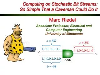
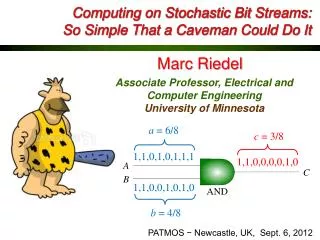
Computing on Stochastic Bit Streams: So Simple That a Caveman Could Do It. Marc Riedel. a = 6/8. c = 3/8. Associate Professor, Electrical and Computer Engineering University of Minnesota. 1,1,0,1,0,1,1,1. b = 4/8. 1,1,0,0,0,0,1,0. 1,1,0,0,1,0,1,0.

Marc Riedel
E N D
Presentation Transcript
Computing on Stochastic Bit Streams:So Simple That a Caveman Could Do It Marc Riedel a = 6/8 c = 3/8 Associate Professor, Electrical and Computer Engineering University of Minnesota 1,1,0,1,0,1,1,1 b = 4/8 1,1,0,0,0,0,1,0 1,1,0,0,1,0,1,0 PATMOS − Newcastle, UK, Sept. 6, 2012
Positional Encodings 75710 = 7·102 + 5·101 +7·100 Human 10101112 = 26 + 24 + 22 + 21 + 20 Computer • A positional representation scheme is compact: 2ndistinct numbers can be represented with n bits. • Operating on this representation is complex.
Multiplication a x b = c • HA: Half adder, 2 basic gates (AND and XOR) • FA: Full adder, 5 basic gates (AND, OR, and XOR) In total 30 gates!
Multiplication a x b = c a = 6/8 c = 3/8 1,1,0,1,0,1,1,1 1,1,0,0,0,0,1,0 1,1,0,0,1,0,1,0 6/8·4/8 = 3/8 b = 4/8 Assume two input bit streams are independent
Representing a Value by a Sequence of Random Bits A real value x in [0, 1] is represented by a sequence of random bits, each of which has probabilityx of being one and probability of 1 − xof being zero. x = 3/7 0,1,0,1,1,0,0
Serial versus Parallel Stochastic Bit Streams x = 3/7 0,1,0,1,1,0, 0 Probabilistic Bundles 0 1 x = 3/7 0 1 1 0 0
Physical Level Nanowire Crossbar (Idealized) A1 A collection of inverters with shuffled outputs! A2 A3 A4
Nanowire Crossbar Array A1 Shuffled AND A2 A3 A4 B1 B2 B3 B4 A4B3 A1B2 A2B4 A3B1
Stochastic Logic combinationalcircuit Probability values are the input and output signals. 4/8 5/8 3/8 4/8 3/8 8/8
Stochastic Logic combinationalcircuit Probability values are the input and output signals. 0,1,1,0,1,0,1,0,… 1,1,0,1,0,1,1,0… 0,1,1,0,1,0,0,0,… 1,0,1,0,1,0,1,0,… 1,0,0,0,1,1,0,0,… 1,1,1,1,1,1,1,1,… serial bit streams
Stochastic Logic Probability values are the input and output signals. 4/8 5/8 3/8 combinationalcircuit 4/8 3/8 8/8 parallel bit streams
Randomness A/D D/A A/D A/D D/A A/D Analog/digital interface with fractional weighting of 1’s. combinationalcircuit parallel bit streams
= c P ( C ) = c P ( C ) = P ( A ) P ( B ) = + - P ( S ) P ( A ) [ 1 P ( S )] P ( B ) = a b = + - s a ( 1 s ) b Arithmetic Operations Multiplication (Scaled) Addition 1 0
Probabilistic Signals deterministic deterministic random Claude E. Shannon1916 –2001 “A Mathematical Theory of Communication” Bell System Technical Journal,1948.
combinationallogic Synthesizing Logic that Computes on Stochastic Bit Streams 0,1,1,0,1,0,1,0,… 1,1,0,1,0,1,1,0,… 0,1,1,0,1,0,0,0,… 1,0,0,0,0,0,1,0,… 1,0,0,0,1,1,0,0,… 1,0,1,1,0,1,1,1,… Applicable to arbitrary arithmetic functions Gamma CorrectionFunction
Stochastic Logic Probability values are the input and output signals. 0.616 combinationalcircuit 0.7
Stochastic Logic t - + 2 0 . 8 t 0 . 8 t 0 . 3 Probability values are the input and output signals. combinationalcircuit Functions of a probability value t.
X1 Independent Random Boolean Variables X2 Y Xn combinationallogic Mathematical Model Random Boolean Variable ?
Bernstein Polynomial Bernstein basis polynomial of degree n Bernstein polynomial of degree n is a Bernstein coefficient
Bernstein Polynomial Obtain Bernstein coefficients from power-form coefficients: Given , we have
Bernstein Polynomial Elevate the degree of the Bernstein polynomial: , we have Given
coefficients in unit interval Example: Converting a Polynomial Power-Form Polynomial Bernstein Polynomial
Synthesizing Circuit to Implement Polynomial Bernstein coefficient Power-Form Polynomial Bernstein polynomialof degree 2 Bernstein basis polynomial Step 1: Convert the polynomial into a Bernstein form.
Synthesizing Circuit to Implement Polynomial Power-Form Polynomial coefficients all in unit interval less than 0 Step 1: Convert the polynomial into a Bernstein form. Step 2: Elevate the Bernstein polynomial until all coefficients are in the unit interval. Step 3: Implement this with “generalized multiplexing.”
Synthesizing Circuit to Implement Polynomial Power-Form Polynomial (Evaluate on t = 1/2) g(1/2) = 1/4 P(Xi=1) = t (= 1/2) P(Zi=1) = bi,3 (Bernstein Coefficient)
Generalized Multiplexing P(Xi=1) = t Independent P(Zi=1) = bi,n (0 ≤ bi,n≤ 1)
Mathematical Contributions • U is the set of polynomials that can be implemented by logical computation on stochastic bit streams. • V is the set of polynomials that can be represented as Bernstein polynomial with coefficients in the unit interval. • W is the set of polynomials g(t) such that Either g(t) ≡ 0 or ≡ 1 Or 0 < g(t) < 1, for all 0 < t < 1, and 0 ≤ g(0), g(1) ≤ 1 Theorem: “Uniform Approximation and Bernstein Polynomials with Coefficients in the Unit Interval” W. Qian, M. Riedel, and I. Rosenberg European Journal of Combinatorics, 2011 Practical Implication: A necessary and sufficient condition on whether polynomials can beimplemented by logical computation on stochastic bit streams. A guarantee that degree elevation will produce Bernsteinpolynomials with coefficients in the unit interval.
Non-Polynomial Functions Find a Bernstein polynomial with coefficients in the unit interval that approximates the non-polynomial g(t). Find real values to minimize Solved by quadratic programming subject to
Example: Gamma Correction Function Coefficients of Degree-6 Bernstein polynomial approximation: b0,6 = 0.0955, b1,6 = 0.7207, b2,6 = 0.3476, b3,6 = 0.9988, b4,6 = 0.7017, b5,6 = 0.9695, b6,6 = 0.9939
Fault Tolerance • Stochastic Encoding • A bit flip does not substantially change the probability: 1010111001 → 1010011001 • Binary Radix Encoding • A bit flip in the most significant bit causes a huge change in the value: (1010)2 → (0010)2 0.6 0.5 10 2
Fault Tolerance Implementing arithmetic function y=x1x2s+x3(1−s) for x1=4/8, x2=6/8, x3=7/8 and s=2/8. 10% noise injection. StochasticImplementation Small error! DeterministicImplementation Large error!
Deterministic v.s. Stochastic Implementation of Gamma correction function with 10% noise injection. Deterministic implementation:37% pixels with errors > 25% 1% 2% 10% Conventional Implementation Stochastic Implementation: no pixels with errors > 25%! Stochastic Implementation
Hardware Cost Comparison • Compare conventional implementation to stochastic implementation of polynomial functions. • Mapped onto FPGA (counting the number of LUTs) • Conventional implementation: 10-bit binary radix • Stochastic implementation: bit stream of length 210
Comparison of Fault Tolerance for Mathematical Functions Sixth-order Maclaurin polynomial approx., 10 bits: sin(x), cos(x), tan(x), arcsin(x), arctan(x), sinh(x), cosh(x), tanh(x), arcsinh(x), exp(x), ln(x+1)
Sequential Constructs What about complex functions such as tanh, exp, and abs?
Sensing Applications Median Filter-Based Image Noise Reduction
Sensing Applications Frame Difference-Based Image Segmentation
Sensing Applications Image Contrast Enhancing
Sensing Applications Kernel Density Estimation-Based Image Segmentation
General Approach for Generating Stochastic Bit Streams R probability to be one 0, 1, 1, 0, 1, … If R < C, output a one; If R ≥ C, output a zero. Comparator C
Types of Random Sources • Psuedorandom Number Generator Linear Feedback Shift Register (expensive) • Physical Random Source Thermal Noises (cheap)
Challenge withPhysical Random Sources cheap Voltage Regulators expensive expensive C2 C1 Suppose many differentprobabilities are needed:{0.2, 0.78, 0.2549, 0.43, 0.671, 0.012, 0.82, …}. It is costly to generate them directly.(many expensive constant values required.)
Opportunity with Physical Random Sources cheap 1,1,0,0,0, … 0,1,0,1,0, … 0,0,1,0,1, … expensive • Independent • Same probability
Solution When we need many different probabilities: {0.2, 0.78, 0.2549, 0.43, 0.671, 0.012, 0.82, …} • Generate a few probabilities directly from physical random sources. • Synthesize combinational logic to generate other probabilities. Probability: Probability of a signal being logical one