Download
1 / 46
490 likes | 625 Views
Professor William Browne School of Veterinary Science and Centre for Multilevel Modelling. Statistical Software at the Centre for Multilevel Modelling (In part a tribute to the work of Jon Rasbash). Acknowledgements.

E N D
Professor William BrowneSchool of Veterinary Science and Centre for Multilevel Modelling Statistical Software at the Centre for Multilevel Modelling (In part a tribute to the work of Jon Rasbash)
Acknowledgements • Colleagues at CMM past and present (Harvey, Fiona, Min, Jon, Pan, Chris, George, Becky, Sophie, Emma, Hilary, Amy & Lisa, Mike, Geoff, Ian, Mary, Paul, Toni, Mousa, Camille, Richard, Mark, Kelvyn and Liz) • Collaborators on the e-STAT project (Dave, Luc, Danius, Paul, Ian, Mark, Mac) • Coders of STAT-JR (Jon, Chris, Danius, Camille, Toni and Bruce) • ESRC for funding so much of my work!
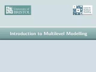
Summary • The distant past • The past • MLwiN • The move (from London to Bristol) • The present • MLPowSim / REALCOM • The future • STAT-JR
So where did it all begin? Q: How does one start writing a statistics package? A: Build it on top of an existing software package! The NANOStat package developed in 1981 by Prof. Mike Healy was a Minitab clone written in RATFOR (Fortran) as something to do with his new computer! Mike worked at LSHTM but also at Rothamsted with Fisher! Recounted writing programs to invert matrices.
NANOStat (1981) • Data represented as a set of columns • Commands took columns, numbers and boxes as arguments • Commands strung together so output from 1 command acts as input to another (became MLwiN macro language) • Software consisted of functions to create columns and several hundred commands. Still sits under MLwiN today!
ML2, ML3 and MLN • Jon worked for Mike at LSHTM and then transferred to Harvey at Institute of Education. • Harvey wrote his IGLS paper in 1986 • ML2 came out in 1988 (written in Fortran) • ML3 followed in 1990 (converted to C code) • MLN followed in 1995 (with new N level algorithms written in C++) • Algorithms very fast for hierarchical models – good matrix routines for block diagonal structures. • Bob Prosser completed the team.
Moving towards MLwiN - Jon • MLwiN was another step change, this time to a Windows based program. • ML2/3/N worked in a sequential way with each command performing an action and then the next etc.… Graphics were limited. • MLwiN in contrast consists of a GUI front-end (written in Visual Basic) and all the objects are dynamic i.e. changing one window should change the contents of other windows. • Jon worked with Bruce Cameron setting up this architecture and Bruce is still involved in STAT-JR.
Moving towards MLwiN – Bill in Bath • I did my MSc. (Comp Stats) in 1995 and used S-Plus and C and BUGS to fit models for my dissertation. • I then did my PhD. (Stats) between 1995 and 1998 supervised by David Draper. My PhD. included much comparison work between methods of fitting multilevel models (Bayesian & frequentist) • I did this using both BUGS and MLwiN • An artefact of the process was writing (limited) MCMC functionality into MLwiN!
MLwiN in 1998 What was good / What was new? • Interactive Equations window • Interactive Graphics • Interactive Trajectories window • Choice of estimation methods • Adaptive Metropolis algorithms
Interactive Equations Window This is the 2011 version but the 1998 version had many of the same features. Could toggle between estimates and symbols. Numbers changing from blue to green on convergence. Clicking on the window would allow model construction – see X variable window.
Interactive Graphics Graphics can instantly update as column content changes. Highlighting of data points passed between graphs. Highlighting can be done at different levels of the data structure
Interactive Trajectories Window Trajectories plot particularly useful for MCMC estimation First software (to my knowledge) to have dynamic chains although they appeared in WinBUGS soon after. Used to joke about taking a coffee break while MCMC ran and chains make you look busy! Click on graph to get diagnostics
Sixway diagnostic plot Plot of chain plus kernel density – code from my MSc! Kernel would show informative priors as well. Time series plots and originally MCSE and summary in bottom 2 boxes. Expanded to 7 boxes later.
MCMC functionality • In 1998 we had implemented Normal, Binomial and Poisson N level models by shoe horning my stand-alone C code into MLwiN in a couple of manic visits to London. • For Normal responses used Gibbs sampling, for others used a mixture of Gibbs and random walk Metropolis including my ad-hoc adapting scheme that persists today. • BUGS used AR sampling instead of MH at the time. • Code was very model specific and optimised so far faster than BUGS as it still is today!
Changes from 1989 to 1999 1989 • Normal response, hierarchical, IGLS algorithm 1999 • Normal, Poisson, Binomial and Multinomial responses • Hierarchical, cross-classified and multiple membership (in IGLS see Rasbash and Goldstein) • IGLS, bootstrapping and MCMC.
Move to the CMM at the IOE in 1998 • CMM in 1998 : Harvey, Jon, Min and Pan • Ian Plewis and Geoff Woodhouse also at IOE • Chris Charlton did summer work in 1998 and 1999 on many of the new windows in the package. • I joined in October 1998 (and lived in Jon’s house for a few months!) • Fiona Steele joined a couple of years later from LSE when Geoff Woodhouse left
Changes to MLwiN in my time at IOE (1998-2003) • Better handling of missing data, categorical variables. • Lots more data manipulation windows. • MCMC functionality for: XC/MM/Spatial CAR models (Browne et al. 2001a) Multilevel Factor Analysis (Goldstein & Browne 2002,2005) Measurement Error (Browne et al 2001b) Multivariate/Mixed responses/Complex variation (Browne 2006) 17
Happy times at a Centre away day and croquet Harvey was taking the photo (includes Mike Healy)
Documentation Part of the success of MLwiN is due to the quality and quantity of the accompanying documentation: • Users Guide in 1998 (Goldstein et al. ~130 pages) By 2003 • Users Guide (Rasbash et al. ~ 250 pages) & MCMC Guide (Browne et al.) & Command guide Today: User’s Guide (314 pages) Supplement (114 pages) MCMC Guide (439 pages) Command guide (114 pages) Huge effort by colleagues in centre on web-based training materials.
Moves are afoot! • In 2003 I moved from London to Nottingham to take a lecturing position. • The grant that would have continued funding me produced the start of the REALCOM software • In 2005 as Harvey retired the centre began the move to Bristol – first Jon then Fiona. • The first LEMMA project began in 2005 and Chris Charlton (re)joined centre. Chris gradually became main coder of MLwiN as Jon took a more managerial role directing centre.
REALCOM • Harvey extended our earlier MCMC work to create the suite of REALCOM functions to cover: • (further) Measurement error modelling • Structural equations models (extending the factor analysis work) • (further) Mixed responses and imputation (REALCOM – IMPUTE) – with input from James and Mike at LSHTM • Harvey wrote REALCOM in MATLAB which was easier to code in but slower. • Jon and Chris put a front end on the software.
Grants at Nottingham! • In 2006 an ESRC grant to look at power calculations in multilevel models (along with MCMC algorithm improvements) began at Nottingham. • This employed Mousa Golalizadeh. • I also was a sponsor of a Wellcome grant on Bayesian modelling of vet (mastitis) data with Martin Green. • In late 2006 I was interviewed for a chair at Bristol vet school and got a chance to rejoin CMM when I arrived in April 2007 at Bristol.
MLPowSim • The power grant resulted in MLPowSim – a program to perform power calculations for multilevel models • Note that Cora Maas (with Joop Hox) did lots of good work in this area. • Program creates MLwiN macro files or R scripts to run via simulation power calculations. • Program developed with two postdocs Mousa and Richard Parker and work continues with new PhD student Toni Price.
MLPowSim • Software freely available from http://seis.bris.ac.uk/~frwjb/esrc.html
MLwiN (2003-) We still develop MLwiN: • The Users guide supplement shows Jon & Chris’s work on improved model specification, model comparison, customised predictions and auto-correlated error modelling. • The last 5 chapters of the MCMC guide shows my work on MCMC algorithm improvements (SMVN, SMCMC, hierarchical centring, parameter expansion and orthogonal parameterisations) see also Browne et al. (2009)
MLwiN – A picture of where we have come Picture courtesy of Becky Pillinger.
Impact – “It’s papers not programs stupid!” MLwiN has over 2,000 citations (since 1998) which represent only a small proportion of actual use in published work. The spread of topics includes: 466 in public health, 150 in statistics/probability 135 in education, 101 in social science, biomed. 86 in health care, 86 in psychiatry, 78 in medicine, 77 in vet science, 63 zoology, 58 ecology, 57 in sport science, 55 behavioural science, several hundred in various forms of psychology.
Jon’s big vision • Jon had been thinking hard on where the software went next. • The frequentist IGLS algorithm was hard to extend further. • WinBUGS showed that MCMC as an algorithm could be extended easily but the difficulty in MLwiN was in extending my MCMC code and possibly relying on the personnel! • The big vision was an all-singing all-dancing system where expert users could add functionality easily and which interoperates with other software. Bruce was developing an underpinning algebra system. • The ESRC LEMMA II and E-STAT grants would enable this to be achieved
2010 – Annus Horribilis • Sadly Jon’s vision didn’t have a happy ending for him following his tragic death last year. • 2010 was a pretty rotten year for CMM as a result although we have now picked up most of the pieces. • Fiona and I (with Harvey and other colleagues support) have taken on Jon’s role to lead the centre and the announcement of the successful bid for LEMMA III (led by Fiona) in 2011, looking at more longitudinal modelling seems like a rebirth. • One ‘phoenix from the flames’ is the STAT-JR package currently developing which is our take on Jon’s vision.
The E-STAT project and STAT-JR STAT-JR developed jointly by LEMMA II and E-STAT Consists of a set of components many of which we have an alpha version for which contains: Templates for model fitting, data manipulation, input and output controlled via a web browser interface. Currently model fitting for 90% of the models that MLwiN can fit in MCMC plus some it can’t including greatly sped up REALCOM templates Some interoperability with MLwiN, WinBUGS, R, Stata and SPSS (written by Camille) Also runmlwin in Stata -> MLwiN written by George
STAT-JR Jon identified 3 groups of users: • Novice practitioners who want to use statistical software that is user friendly and maybe tailored to their discipline • Advanced practitioners who are the experts in their fields and also want to develop tools for the novice practitioners • Algorithm Developers who want their algorithms used by practitioners. • See http://www.cmm.bristol.ac.uk/research/NCESS-EStat/news.shtml for details of Advanced User’s guide for STAT-JR
STAT-JR component based approach Below is an early diagram of how we envisioned the system. Here you will see boxes representing components some of which are built into the STAT-JR system. The system is written in Python with currently a VB.net algebra processing system. A team of coders (currently me, Chris, Danius, Camille and Bruce) work together on the system.
Templates • Consist of a set of code sections for advanced users to write. For a model template it consists of at least: • an invars method which specifies inputs and types • An outbug method that creates (BUGS like) model code for the algebra system • An (optional) outlatex method can be used for outputting LaTeX code for the model. Other optional functions required for more complex templates
Regression 1 Example from EStat.Templating import * from mako.template import Template as MakoTemplate import re class Regression1(Template): 'A model template for fitting 1 level Normal multiple regression model in E-STAT only. To be used in documentation.' tags = [ 'model' , '1-Level' ] invars = ''' y = DataVector('response: ') tau = ParamScalar() sigma = ParamScalar() x = DataMatrix('explanatory variables: ') beta = ParamVector() beta.ncols = len(x) ''' outbug = ''' model{ for (i in 1:length(${y})) { ${y}[i] ~ dnorm(mu[i], tau) mu[i] <- ${mmult(x, 'beta', 'i')} } # Priors % for i in range(0, x.ncols()): beta${i} ~ dflat() % endfor tau ~ dgamma(0.001000, 0.001000) sigma <- 1 / sqrt(tau) } ''' outlatex = r''' \begin{aligned} \mbox{${y}}_i & \sim \mbox{N}(\mu_i, \sigma^2) \\ \mu_i & = ${mmulttex(x, r'\beta', 'i')} \\ %for i in range(0, len(x)): \beta_${i} & \propto 1 \\ %endfor \tau & \sim \Gamma (0.001,0.001) \\ \sigma^2 & = 1 / \tau \end{aligned} '''
Equations for model and model code Note Equations use MATHJAX and so underlying LaTeX can be copied and paste. The model code is based around the WinBUGS language with some variation. This is a more complex template for 2 level models.
Model code in detail model { for (i in 1:length(normexam)) { normexam[i] ~ dnorm(mu[i], tau) mu[i] <- cons[i] * beta0 + standlrt[i] * beta1 + u[school[i]] * cons[i] } for (j in 1:length(u)) { u[j] ~ dnorm(0, tau_u) } # Priors beta0 ~ dflat() beta1 ~ dflat() tau ~ dgamma(0.001000, 0.001000) tau_u ~ dgamma(0.001000, 0.001000) } For this template the code is, aside from the length function, standard WinBUGS model code.
Output of generated C++ code The package can output C++ code that can then be taken away by software developers and modified.
Output from the E-STAT engine Here the six-way plot functionality is in part taken over to STAT-JR after the model has run. In fact graphs for all parameters are calculated and stored as picture files so can be easily viewed quickly.
Interoperability with WinBUGS Interoperability in the user interface is obtained via a few extra inputs. In fact in the template code user written functions are required for all packages apart from WinBUGS. The transfer of data between packages is however generic.
Output from WinBUGS with multiple chains STAT-JR generates appropriate files and then fires up WinBUGS. Multiple Chains are superimposed in the sixway plot output.
Interoperability with R R interoperability for a 2-level model can use the glmer or the mcmcglmm functions
Output from R Currently the R output is displayed but other files including the scripts are stored in a directory and will be made available when the e-Book work is done.
Other templates - TemplateXYlabel Can make use of Python’s fantastic graphics! Or potentially other package graphics via interoperability.
The E-STAT project – still to come We have lots of work to do: • Parallel processing. • E-books. • Optimising code generation. • Improving algebra system. • Suites of templates for missing data and social network models. • Interoperability with SAS and hooking up more templates for other packages.