Machine Learning

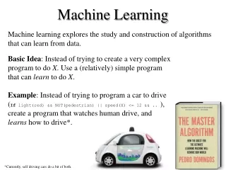
Machine Learning • Learning is “any change in a system that allows it to perform better the second time on repetition of the same task or on another task drawn from the same population” (Herbert Simon, 1983) • Different types of AI learning models • Inductive learning • Explanation based learning • Supervised learning • Unsupervised learning • Parallel distributed processing (PDP) models • Neural networks

An Inductive Learning Framework • Data and goals of learning task • Representation of learned knowledge • Specific instance of concept “ball” • size(obj1, small) Ù color(obj1,red) Ù shape(obj1, round) • General concept “ball” • size(X, Y) Ù color(X,Z) Ù shape(X, round) • Operations on data • Concept space • Combination of representations and operations • Heursitic search

Version Space • Version space is a set of concept descriptions consistent with the training data • Generalization and specialization • shape(box, cube) → shape(X, cube) • size(X, large) Ù shape(X, round) → shape(X, round) • color(X, blue) Ù shape(X, cube) → color(X, blue) Ù (shape(X, cube) Ú shape(X, rectangle)) • “Theory” of Generalization • Given predicate sentences p and q, let P and Q be the set of all sentences that satisfy p and q, respectively. Expression p is more general that q iif. P Ê Q

Concept Space Searches • Specific to general • Goal is to create a set S (hypotheses) of maximally specific generalizations • Maintain set NL of previously observed negative examples (initially empty) • Initialize S to first positive training instance in PG •  p : p Î PG • s : s Î S, if s ≠ p, let s = most specific generalization that matches p • Remove from S all hypotheses more general than other hypotheses in S • Remove from S all hypotheses that match a previously observed negative in NL •  n : n Î NG • Add n to NL • s : s Î S  s = n, remove s from S • General to specific • Goal is to create a set G of maximally general concepts • Maintain set PL of previously observed positive examples • Initialize G to the most general concepts •  n : n Î NG • g : g Î G, if g = n, let g = most general specializations that do not match n • Remove from G all hypotheses more specific than other hypotheses in G • Remove from G all hypotheses that fail to match a previously observed positive in PL •  p : p Î PG • Add p to PL • g : g Î G  g ≠ p, remove g from G

Concept Space Search Examples X = {small, large} Y = {red, white, blue} Z = {ball, cube, brick} S: {} Positive: obj(small, red, ball) S: {obj(small, red, ball)} Positive: obj(small, white, ball) S: {obj(small, Y, ball)} Positive: obj(large, blue, ball) S: {obj(X, Y, ball)} Specific => General G {obj(X, Y, Z)} Negative: obj(small, red, brick) G: {obj:(large, Y, Z), obj(X, white, Z), obj(X, blue, Z), Positive: obj(large, white, ball) obj(X, Y, ball), obj(X, Y, cube)} G: {obj(large, Y, Z), obj(X, white, Z), obj(X, Y, ball)} Negative: obj(large, blue, cube) G: {obj(large, white, Z), obj(X, white, Z), obj(X, Y, ball)} Positive: obj(small, blue, ball) G: {obj(X, Y, ball)} General => Specific

Version Space Convergence • Generalization and specialization lead to version space convergence • Specialization of general models • Generalization of specific models • Candidate Elimination Algorithm • Bi-directional search - combines previous two search techniques • If G = S and |S| = |G| = 1, then a single goal concept has been found • Otherwise, there is no single concept that covers all positive instances and none of the negative instances http://www2.cs.uregina.ca/~hamilton/courses/831/notes/ml/vspace/3_vspace.html

Candidate Elimination Algorithm G: {obj(X, Y, Z)} Positive: obj(small, red, ball) S: {} G: {obj(X, Y, Z)} Negative: obj(small, blue, brick) S: {obj(small, red, ball)} G: {obj(X, red, Z), obj(X, Y, ball)} Positive: obj(large, red, ball) S: {obj(small, red, ball)} G: {obj(X, red, Z), obj(X, Y, ball)} Negative: obj(large, red, cube) S: {obj(X, red, ball)} G: {obj(X, red, ball)} S: {obj(X, red, ball)}

Explanation-Based Learning • Explanation-Based Algorithm • Target concept • Agent must find an effective definition of this concept • Training example • Domain theory (premise(X) → conclusion(X)) • liftable(X)  container(X) → cup(X) • part(Z, W)  concave(W)  points_up(W) → container(Z) • light(Y)  part(Y, handle) → liftable(Y) • small(A) → light(A) • made_of(Z, feathers) → light(A) • Operational criteria • Means of describing the form of concept definitions

Explanation-Based Learning Example Specific and Generalized Proof Trees cup(obj1) cup(obj1) small(obj1) part(obj1, handle) owns(bob, obj1) part(obj1, bottom) part(obj1, bowl) points_up(bowl) concave(bowl) color(obj1, red) liftable(obj1) container(obj1) light(obj1) part(obj1, handle) part(obj1, bowl) points_up(bowl) concave(bowl) small(obj1) cup(X) liftable(X) container(X) light(obj1) part(X, handle) part(X, W) points_up(W) concave(W) small(X)

Benefits of Explanation-Based Learning • Domain theory allows the learner to select relevant aspects of the training instance • Ignores irrelevant aspects such as color of the cup • EBL forms generalizations that we know to be relevant to specific goals and consistent with the domain theory • Many instances may allow numerous possible generalizations that are either meaningless or wrong • Allows the learner to learn from a single instance • Allows the learner to hypothesize unstated relationships between goals and experiences

Unsupervised Learning • Supervised learning assumes the existence of an external method to correctly classify training data • Unsupervised learning require that the learner evaluate concepts on its own • AM is an early example of a discovery program • Discovered natural numbers by modifying its notion of “bags,” or multisets. • Figured out addition, multiplication, division, and prime numbers by evaluating “interesting” concepts • Failed beyond rudimentary number theory – space grew combinatorially and percentage of interesting concepts diminished

Concept Clustering • The goal of the clustering problem is to organize a collection of objects into some hierarchy of classes that meet some standard of quality • Necessary to have some means of measuring similarity between objects • Numeric taxonomy represents objects as collections of features and assigns numeric values to these features • Similarity metric treats object as a point in n-dimensional space, where n is the number of features. Similarity between two objects is thus the Euclidean distance between them

Agglomerative Clustering • Bottom-up approach to the clustering problem • Examine all pairs of objects, and make the pair with the highest degree of similarity a cluster • Define the features of this cluster as some function (i.e. average) of the features of the members and replace the component objects with this definition • Repeat until all objects have been reduced to a single cluster • Difficult to compare objects defined using symbolic features rather than numeric features • Define similarity as a proportion of common features • However does not adequately take into account underlying semantic knowledge or take into account goals or background knowledge • Traditional algorithms are extensional, enumerate all members. No intensional definition to classify both known and future members

Parallel Distributed Processing (PDP) • Also known as subsymbolic approaches/models • View intelligence as the behavior of a collection of large numbers of simple interacting components • Symbolic systems suffer from brittleness • Encompasses phenomena related to the nature of a two-value system • Human performance degrades as a problem gets harder, but almost always generates some answer; expert systems either perform perfectly or not at all • Neural networks • Connectionalist approach inspired by biological brains

Neural Networks • Neurons • Inputs values: xi • Usually discrete, real values, or within {0, 1} or {-1, 1} • Weights: wi • Usually real valued • Activation values • Output of the neuron • Activation function: F • Neural network • Network topology • Learning algorithm • Environment

Simple Neural Networks • McCulloch-Pitts Neuron (McCulloch and Pitts, 1943) • Inputs are either +1 or -1, activation function multiplies each input by its weight as sums the result • If the sum is greater than or equal to 0, the output is 1. Otherwise the output is 0 Output X  Y X  Y ⌐X Weight +1 +1 -2 +1 +1 -1 -1 Inputs X Y +1 X Y +1 X

Perceptrons • Devised by Frank Rosenblatt in the late 1950s • A single-layer network where all inputs and activation values are either 0 or 1, and the weights are real valued • Activation function is a simple linear threshold • 1 if ∑ xiwi > t • 0 otherwise • Supervised learning, perceptron changes weights based on correct results • If output is correct, do nothing • If output is 0 and should be 1, increment weights on the active lines (input of 1) by some amount d. • If output is 1 and should be 0, decrement weights on the active lines by some amount d.

Limits of Perceptrons • Single-layer networks are only capable of learning classes that are linearly separable • For example, exclusive-or is not linearly separable, and thus cannot be represented by a perceptron • For any n-dimensional space, a classification is linearly separable if these groups can be separated with a single n-1 dimensional hyperplane Y 1 X xor Y = 0 X xor Y = 1 X 0 1

Modern Machine Learning Topics • Asymptotic Model Selection for Naive Bayesian Networks • Dimension Reduction in Text Classification with Support Vector Machines • Stability of Randomized Learning Algorithms • Diffusion Kernels on Statistical Manifolds • Multiclass Boosting for Weak Classifiers • Denoising Source Separation • Learning with Decision Lists of Data-Dependent Features • Generalization Bounds and Complexities Based on Sparsity and Clustering for Convex Combinations of Functions from Random Classes • Characteristics of a Family of Algorithms for Generalized Discriminant Analysis of Undersampled Problems Journal of Machine Learning Research, http://jmlr.csail.mit.edu

Machine Learning