Machine Learning

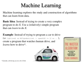
1. Machine Learning Machine learning explores the study and construction of algorithms  that can learn from data. Basic Idea: Instead of trying to create a very complex program to do X. Use a (relatively) simple program that can learn to do X. Example: Instead of trying to program a car to drive (If light(red) && NOT(pedestrian) || speed(X) <= 12 && .. ), create a program that watches human drive, and learns how to drive*. *Currently, self driving cars do a bit of both.

2. Why Machine Learning I Why do machine learning instead of just writing an explicit program? • It is often much cheaper, faster and more accurate. • It may be possible to teach a computer something that we are not sure how to program. For example: • We could explicitly write a program to tell if a person is obese If (weightkg /(heightm heightm)) > 30, printf(“Obese”) • We would find it hard to write a program to tell is a person is sad However, we could easily obtain a 1,000 photographs of sad people/ not sad people, and ask a machine learning algorithm to learn to tell them apart.

3. Validation Data Training Data If we have the luxury of having lots of data. We can divide the data into Validation Data and Training data. The Validation Data we hid from ourselves, and we use the Training Data to pick our classification model, to set the K in K-Nearest neighbor, to figure out our training policy etc. Only when we have 100% finish all of this do we finally test on the Validation Data. We might even give the Validation Data to someone else at the beginning, and have them test our model.

4. The Classification Problem (informal definition) Katydids Given a collection of annotated data. In this case 5 instances Katydids of and five of Grasshoppers, decide what type of insect the unlabeled example is. Grasshoppers Katydid or Grasshopper?

5. The Classification Problem (informal definition) Canadian Given a collection of annotated data. In this case 3 instances Canadian of and 3of American, decide what type of insect the unlabeled example is. American Canadian or American?

6. Blame Canada

7. For any domain of interest, we can measure features Color {Green, Brown, Gray, Other} Has Wings? Abdomen Length Thorax Length Antennae Length Mandible Size Spiracle Diameter Leg Length

8. What features can we cheaply measure from coins? Diameter Thickness Weight Electrical Resistance ? Probably not color or other optical features.

9. The Ideal Case In the best case, we would find a single feature that would strongly separate the coins. Diameter is clearly such a feature for the simpler case of pennies vs. quarters. Nominally 19.05 mm Nominally 24.26 mm Decision threshold 20mm 25mm

10. Usage Once we learn the threshold, we no longer need to keep the data. When an unknown coin comes in, we measure the feature of interest, and see which side of the decision threshold it lands on. IF diameter(unknown_coin) < 22 coin_type = ‘penny’ ELSE coin_type = ‘quarter’ END ? Decision threshold 20mm 25mm

11. Let us revisit the original problem of classifying Canadian vs. American Quarters Which of our features (if any) are useful? Diameter Thickness Weight Electrical Resistance I measured these features for 50 Canadian and 50 American quarters….

12. Diameter Here I have 99% blue on the right side, but the left side is about 50/50 green/blue. 1

13. Thickness Here I have all green on the left side, but the right side is about 50/50 green/blue. 2

14. 3 Weight The weight feature seem very promising. It is not perfect, but the left side is about 92% blue, and the right side about 92% green

15. 4 The electrical resistance feature seems promising. Again, it is not perfect, but the left side is about 89% blue, and the right side about 89% green. Electrical Resistance

16. Diameter We can try all possible pairs of features. {Diameter, Thickness} {Diameter, Weight} {Diameter, Electrical Resistance} {Thickness, Weight} {Thickness, Electrical Resistance} {Weight, Electrical Resistance} This combination does not work very well. Thickness 1 2 1,2

17. Diameter 1 3 1,3 Weight

18. For brevity, some combinations are omitted • Let us jump to the last combination…

19. 3 4 3,4 Weight Electrical Resistance

20. 5 0 Diameter -5 -10 5 5 0 0 -5 -5 -10 Thickness 1 2 3 We can also try all possible triples of features. {Diameter, Thickness, Weight} {Diameter, Thickness, Electrical Resistance} etc This combination does not work that well. 1,2 1,3 2,3 Weight 1,2,3

21. Diameter Thickness 1 2 3 4 1,2 1,3 2,3 1,4 2,4 3,4 Weight 1,2,3 1,2,4 1,3,4 2,3,4 1,2,3,4 Electrical Resistance

22. Given a set of N features, there are 2N -1 feature subsets we can test. In this case, we can test all of them (exhaustive search), but in general, this is not possible. • 10 features = 1,023 • 20 features = 1,048,576 • 100 features = 1,267,650,600,228,229,401,496,703,205,376 We typically resort to greedy search. Greedy Forward Section Initial state: Empty Set: No features Operators: Add a single feature. Evaluation Function: K-fold cross validation. 1 2 3 4 1,2 1,3 2,3 1,4 2,4 3,4 1,2,3 1,2,4 1,3,4 2,3,4 1,2,3,4

23. The Default Rate How accurate can we be if we use no features? The answer is called the Default Rate, the size of the most common class, over the size of the full dataset. Examples: I want to predict the sex of some pregnant friends babies. The most common class is ‘boy’, so I will always say ‘boy’. I do just a tiny bit better than random guessing. I want to predict the sex of the nurse that will give me a flu shot next week. The most common class is ‘female’, so I will say ‘female’. No features

24. Greedy Forward Section Initial state: Empty Set: No features Operators: Add a feature. Evaluation Function: K-fold cross validation. 1 2 3 4 100 80 1,2 1,3 2,3 1,4 2,4 3,4 60 40 1,2,3 1,2,4 1,3,4 2,3,4 20 0 {} 1,2,3,4

25. Greedy Forward Section Initial state: Empty Set: No features Operators: Add a feature. Evaluation Function: K-fold cross validation. 1 2 3 4 100 80 1,2 1,3 2,3 1,4 2,4 3,4 60 40 1,2,3 1,2,4 1,3,4 2,3,4 20 0 {} {3} 1,2,3,4

26. Greedy Forward Section Initial state: Empty Set: No features Operators: Add a feature. Evaluation Function: K-fold cross validation. 1 2 3 4 100 80 1,2 1,3 2,3 1,4 2,4 3,4 60 40 1,2,3 1,2,4 1,3,4 2,3,4 20 0 {} {3} {3,4} 1,2,3,4

27. Greedy Forward Section Initial state: Empty Set: No features Operators: Add a feature. Evaluation Function: K-fold cross validation. 1 2 3 4 100 80 1,2 1,3 2,3 1,4 2,4 3,4 60 40 1,2,3 1,2,4 1,3,4 2,3,4 20 0 {} {3} {3,4} {1,3,4} 1,2,3,4

28. 10 9 8 7 6 Left Bar 5 4 3 2 1 1 2 3 4 5 6 7 8 10 9 Right Bar Feature Generation I Sometimes, instead of (or in addition to) searching for features, we can make new features out of combinations of old features in some way. Recall this “pigeon problem”. … We could not get good results with a linear classifier. Suppose we created a new feature…

29. 10 9 8 7 6 Left Bar 5 4 3 2 1 1 2 3 4 5 6 7 8 10 9 Right Bar Feature Generation II Suppose we created a new feature, called Fnew Fnew = |(Right_Bar – Left_Bar)| Now the problem is trivial to solve with a linear classifier. 1 2 3 4 5 6 7 8 10 9 0 Fnew

30. Feature Generation III We actually do feature generation all the time. Consider the problem of classifying underweight, healthy, obese. It is a two dimensional problem, that we can approximately solve with linear classifiers. But we can generate a feature call BMI, Body-Mass Index. BMI = height/ weight2 This converts the problem into as easy 1D problem 18.5 24.9 BMI

31. Lets talk some more about features.

32. (Western Pipistrelle (Parastrellushesperus) Photo by Michael Durham

33. We can easily measure two features of bat calls. Their characteristic frequency and their callduration Characteristic frequency Call duration Western pipistrelle calls

37. Quick Review We have seen the simple linear classifier. One way to generalize this algorithm is to consider other polynomials…

38. Quick Review Another way to generalize this algorithm is to consider piecewise linear decision boundaries.

39. Quick Review 10 9 8 7 6 Left Bar 5 4 3 2 1 1 2 3 4 5 6 7 8 10 9 Right Bar There really are datasets for which the more expressive models are better…

41. Underfitting A good model Overfitting

42. Overfitting How do we chose the right model? It is tempting to say: Test all models, using cross validation, and pick the best one. However, this has a problem. If we do this, we will find that a more complex model will almost certainly do better on our training set, but will worse when we deploy it. This is overfitting, a major headache in data mining.

43. 10 9 8 7 6 5 4 3 2 1 1 2 3 4 5 6 7 8 9 10 Imagine the following problem: There are two features, the Y-axis is irrelevant to the task (but we do not know that) and scoring above 5 on the X-axis means you are red-class, otherwise you are blue class. Again, we do not know this, as we prepare to build a classifier.

44. 10 9 8 7 6 5 4 3 2 1 1 2 3 4 5 6 7 8 9 10 Suppose we had a billion exemplars, what would we see? In this case, we would expect to learn a decision boundary that is almost exactly correct.

45. 10 9 8 7 6 5 4 3 2 1 1 2 3 4 5 6 7 8 9 10 With less data, our decision boundary makes some errors. In the green area, it claims that instances are red, when they should be blue. In the pink area, it claims that instances are blue, when they should be red. However, overall it is doing a pretty good job.

46. 10 9 8 7 6 5 4 3 2 1 1 2 3 4 5 6 7 8 9 10 If we allow a more complex model, we will end up doing worse when we deploy the model, even though it performs well now. In the green area, it claims that instances are red, when they should be blue. In the pink area, it claims that instances are blue, when they should be red.

47. 10 9 8 7 6 5 4 3 2 1 1 2 3 4 5 6 7 8 9 10 If we allow a more complex model, we will end up doing worse when we deploy the model, even though it performs well now. In the green area, it claims that instances are red, when they should be blue. In the pink area, it claims that instances are blue, when they should be red.

48. Training Data Complexity of the model

49. Training Data Validation Data Complexity of the Model

50. 10 10 9 9 8 8 7 7 6 6 5 5 4 4 3 3 2 2 1 1 1 1 2 2 3 3 4 4 5 5 6 6 7 7 8 8 9 9 10 10 Rule of Thumb: When doing machine learning, prefer simpler models. This is called Occam's Razor. Complexity of the Model