Download
1 / 34
340 likes | 462 Views
Two-Stage Treatment Strategies Based On Sequential Failure Times. Peter F. Thall Biostatistics Department Univ. of Texas, M.D. Anderson Cancer Center. Designed Experiments: Recent Advances in Methods and Applications Cambridge, England August 2008. Joint work with Leiko Wooten, PhD

E N D
Two-Stage Treatment Strategies Based On Sequential Failure Times Peter F. Thall Biostatistics Department Univ. of Texas, M.D. Anderson Cancer Center Designed Experiments: Recent Advances in Methods and Applications Cambridge, England August 2008
Joint work with Leiko Wooten, PhD Chris Logothetis, MD Randy Millikan, MD Nizar Tannir, MD The basis for a multi-center trial comparing 2-stage strategies for Metastatic Renal Cell Cancer
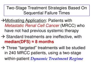
A Metastatic Renal Cancer Trial • Entry Criteria: Patients withMetastatic Renal Cell Cancer (MRCC) who have not had previous systemic therapy • Standard treatments are ineffective, with median(DFS) approximately 8 months Three “targeted” treatments will be studied in 240 MRCC patients, using a two-stage within-patient Dynamic Treatment Regime
A Within-Patient Two-Stage Treatment Assignment Algorithm (Dynamic Treatment Regime) Stage1 At entry, randomize the patient among the stage 1 treatment pool {A1,…,Ak} Stage 2 If the 1st failure is disease worsening (progression of MRCC) & not discontinuation, re-randomize the patient among a set of treatments {B1,…,Bn} not received initially “Switch-Away From a Loser”
Frontline Salvage Strategy A B C • B = (A, B) • C = (A, C) • A = (B, A) • C = (B, C) • A = (C, A) • B = (C, B)
Selection Trials: Screening New Treatments - Randomize patients among experimental treatment regimes E1,…, Ek - Evaluate each patient’s outcome(s) - Select the “best” treatment E[k] that maximizes a summary statistic quantifying treatment benefit A selection design does not test hypotheses It does not detect a given improvement over a null value with given test size and power E.g. with k=3, in the “null” case where q1 = q2 = q3 each Ej is selected with probability .33 (not .05 or some smaller value)
Goal of the Renal Cancer Trial Select the two-stage strategy having the largest “average” time to second treatment failure (“overall failure time”) With 6 strategies: In the “null” case where all strategies give the same overall failure time, each strategy is selected with probability 1/6 = .166
Higher Mathematics Stage1 treatment pool = {A1,…,Ak} Stage 2 treatment pool = {B1,…,Bn} kxn = # possible 2-stage strategies N/k = effective sample size to estimate each frontline rx effect N/(kn) = effective sample size to estimate each two-stage strategy effect
Higher Mathematics Example : If k=3, n=3 with “switch-away” within patient rule, and N=240 2x3 = 6 = # possible 2-stage strategies 240/3 = 80 = effective sample size to estimate each frontline rx effect 240/6 = 40 = effective sample size to estimate each two-stage strategy effect
Outcomes TD = time of discontinuation S1 = time from start of stage 1 of therapy of 1st disease worsening S2 = time from start of stage 2 of therapy to 2nd treatment failure d = delay between 1st progression and start of 2nd stage of treatment
Outcomes T1 = Time to 1st treatment failure T2 = Time from 1st disease worsening to 2nd treatment failure T1 + T2 = Time of 2nd treatment failure (provided that the 1st failure was not a discontinuation)
Unavoidable Complications Because disease is evaluated repeatedly (MRI, PET),either T1 or T1 + T2may be interval censored There may be a delay between 1st failure and start of stage 2 therapy T1 may affect T2 The failure rates may change over time (they increase for MRC)
Delay before start of 2nd stage rx Discontinuation Start of stage 2 rx
T2,1 = Time from 1st progression to 2nd treatment failure if it occurs during the delay interval before stage 2 therapy is begun T2,2 = Time from 1st progression to 2nd treatment failure if it occurs after stage 2 therapy has begun
A Simple Parametric Model Weib(a,x) = Weibull distribution with meanm(a,x) = ea G(1+e-x), for real-valued a and x [ T1 | A ] ~ Weib(aA,xA) [ T2,1 | A,B, T1] ~ Exp{ gA+bA log(T1) } [ T2,2 | A,B, T1] ~ Weib( gA,B+bA log(T1), xA,B)
Mean Overall Failure Time T = T1 + Y1,W T2 mA,B(q) = E{ T| (A,B)} = E(T1) + Pr(Y1,W =1) E(T2) Mean time to 1st failure Pr(1st failure is a Disease Worsening) Mean time to 2nd failure
Criteria for Choosing a Best Strategy Mean{ mA,B(q) | data }: B-Weib-Mean 2. Median{ mA,B(q) | data }: B-Weib-Median 3. MLE of mA,B(q) under simple Exponential: F-Exp-MLE 4. MLE of mA,B(q) under full Weibull: F-Weib-MLE
A Tale of Four Designs Design 1 (February 21, 2006) N=240, accrual rate a = 12/month 20 month accrual + 18 mos addt’l FU Stage 1 pool = {A,B,C,D} 12 strategies (A,B), (A,C), (A,D), (B,A), (B,C), (B,D), (C,A), (C,B), (C,D), (D,A), (D,B), (D,C) Drop-out rate .20 between stages (240/12) x .80 = 16 patients per strategy
A Tale of Four Designs Design 2 (April 17, 2006) Following “advice” from CTEP, NCI : N = 240, a = 9/month (“more realistic”) Stage 1 pool = {A,B} (C, D not allowed as frontline) Stage 2 pool = {A,B,C,D} 6 strategies : (A,B), (A,C), (A,D), (B,A), (B,C), (B,D) (240/6) x .80 = 32 patients per strategy
A Tale of Four Designs An Interesting Property of Design 2 Stage 1 may be thought of as a conventional phase III trial comparing A vs B with size .05 and power .80 to detect a 50% increase in median(T1), from 8 to 12 months, embedded in the two-stage design However, the design does not aim to test hypotheses. It is a selection design.
A Tale of Four Designs Design 3 (January 3, 2007) CTEP was no longer interested, but several Pharmas now VERY interested N = 360, a = 12/month, 3 new treatments Stage 1 rx pool = Stage 2 rx pool = {a,s,t} 6 strategies (different from Design 2) : (a,s), (a,t), (s,a), (s,t), (t,a), (t,s) (360/6) x .80 = 48 patients per strategy
A Tale of Four Designs Design 4 (May 15, 2007) Question: Should a futility stopping rule be included, in case the accrual rate turns out to be lower than planned? Answer: Yes!! “Weeding” Rule: When 120 pats. are fully evaluated, stop accrual to strategy (a,b) if Pr{ m(a,b) < m(best) – 3 mos | data} > .90
A Tale of Four Designs Applying the Weeding Rule when 120 patients have been fully evaluated
Establishing Priors q has 28 elements, but the 6 subvectors are qA,B= (n1,A, n2,A,B , aA , xA, gA, bA , aA,B , xA,B) Pr(Dis. Worsening)Reg. of T2 on T1 Weib pars of T1 Weib pars of T2 The qA,B’s are exchangeable across the 6 strategies, so they have the same priors
Establishing Priors n1,A ,n2,A,B~ iid beta(0.80, 0.20) based on clinical experience aA , xA, gA, bA , aA,B , xA,B ~ indep. normal priors Prior means: We elicited percentiles of T1 and [ T2 | T1 = 8 mos], & applied the Thall-Cook (2004) least squares method to determine means Prior variances: We set var{exp(aA)} = var{exp(xA)} = var{exp(xA,B)} = 100 Assuming Pr(Disc. During delay period) = .02 E(mA,B) = 7.0 mos & sd(mA,B) = 12.9
Computer Simulations Simulation Scenarios specified in terms of z1(A) = median (T1 | A) and z2(A,B) = median { T2,2 | T1 = 8, (A,B) } Null values z1 = 8 and z2 = 3 z1 = 12 Good frontline z2 = 6 Good salvage z2 = 9 Very good salvage
Simulations: No Weeding Rule In terms of the probabilities of correctly selecting superior strategies, F-Weib-MLE ~ B-Weib-Median > B-Weib-Mean >> F-Exp-MLE
Sims With Weeding Rule • Correct selection probabilities are affected only very slightly • There is a shift of patients from inferior strategies to superior strategies – but this only becomes substantial with lower accrual rates
Future Research / Extensions Distinguish betweendrop-out and other types of discontinuation and conduct “Informative Drop-Out” analysis Account forpatient heterogeneity Correct forselection biaswhen computing final estimates Accommodatemore than two stages