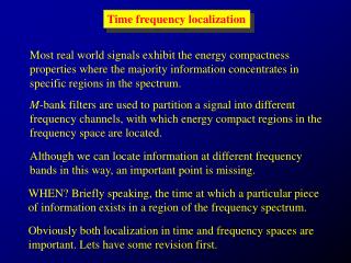
Time frequency localization

Time frequency localization Most real world signals exhibit the energy compactness properties where the majority information concentrates in specific regions in the spectrum. M-bank filters are used to partition a signal into different frequency channels, with which energy compact regions in the frequency space are located. Although we can locate information at different frequency bands in this way, an important point is missing. WHEN? Briefly speaking, the time at which a particular piece of information exists in a region of the frequency spectrum. Obviously both localization in time and frequency spaces are important. Lets have some revision first.

Filter , convolution and Transform x(t) h(t-t) y(t)

Filter , convolution and Transform x(t) is the input signal h(t) is the impulse response of the filter. y(t) is the filter output if h(t) is shifted continuously, y(t) is also continuous For a particular instance h(t - t), y(t) is the projection of x(t) on h(t - t) y(t) = < x(t) , h(t - t) > (dot product) h(t) = ejwt ---> Fourier Transform

Time Frequency Localization f(t) Short time Fourier Transform h(t-b)

Time Frequency Localization h(t-b) t ejwt w(t-b) t

Time Frequency Localization What is the width of the window ? What is w(t) ? Should it be a simple on/off function?

Time Frequency Localization What is the width of the window ? What is w(t) ? Should it be a simple on/off function? If the width is too wide, the time resolution is poor, but frequency resolution is good i.e., same spectrum will be assumed over a long time duration

Time Frequency Localization What is the width of the window ? What is w(t) ? Should it be a simple on/off function? If the width is too wide, the time resolution is poor, but frequency resolution is good i.e., same spectrum will be assumed over a long time duration If the width is too short, the frequency resolution is poor, but time resolution is good i.e., not possible to discriminate small difference in frequency

t 0 1 2 3 4 5 6 7 8 9 10 11 12 13 14 15

t 0 1 2 3 4 5 6 7 8 9 10 11 12 13 14 15 t 0 1 2 3 4 5 6 7 8 9 10 11 12 13 14 15

t 0 1 2 3 4 5 6 7 8 9 10 11 12 13 14 15 t 0 1 2 3 4 5 6 7 8 9 10 11 12 13 14 15 t 0 1 2 3 4 5 6 7 8 9 10 11 12 13 14 15

1.y shifted by b units. 2.y stretched by ‘a’ times if a>1 3.y compress by ‘a’ times if a<1

A stretch in time window corresponds to a compression in the frequency window and vice versa

Time and frequency windows Frequency window Short time window: Long frequency window Long time window: Short frequency window Time window

x(t) Poor Good Good Poor Time localization Frequency localization

Time and frequency windows To detect low frequency content, a large time window is required for good frequency localization To detect high frequency content, a small time window is required for good time localization

Wavelet Family Consider a waveform scaled by ‘s’ and shifted by ‘t’ The larger the value of s, the more the waveform is compressed. The waveform is shifted to the left for positive t. For discrete signal, let The family has two groups, one generated from a mother and the other from a father wavelets.

Wavelet Transform An arbitrary can be transformed into the space formed by members of a wavelet family An inverse transform is also available.

Simple Wavelet : Harr The Harr father wavelet function is a unit step of length 1. It generates a family of scaling functions as shown below: k=0 k=1 k=2 k=3 j=2 k=0 k=1 j=1 The father j=0 k=0 0 1

Simple wavelet : Harr The Harr mother wavelet function is a bipolar [-1,1] unit step of length 0.5. It generates a family of wavelet functions as shown below: k=0 k=1 k=2 k=3 j=2 k=0 k=1 j=1 The mother j=0 k=0 0 1

Simple Wavelet : Harr Scaling functions are like Low Pass Filter. Approximating a waveform f(t) with the set of scaling functions for certain value of ‘j’ gives the coarse form of f(t) at the resolution denoted by ‘j’. f0(t) f(t) 0 1 2 0 1 2 f1(t) ‘j’ must be large enough to capture all the details in f(t). 0 1 2

Wavelet family: Scaling and Wavelet functions Pure use of scaling function to approximate a waveform is viable but not efficient. Very often the scale has to be very fine to capture all the details, resulting in many coefficients. The wavelet functions are like a set of high pass filter which captures the difference between two resolutions (i.e. two values of j). Let Sj represent the space corresponding to scale ‘j’,

Wavelet family: Scaling and Wavelet functions In another words, a high resolution subspace at level ‘j’ can be formed by combining a lower resolution subspaces at ‘j-1’, i.e., We have

Similarly, Multiresolution analysis An important feature of scaling functions: Each can be derived from translation of double-frequency copies of itself, as It means that a scaling function can be built from higher frequency (resolution) replicas of itself. This is known as Multiresolution analysis.

Multiresolution analysis Similar important feature of wavelet functions: Each can be derived from translation of double-frequency copies of scaling function, as It means that a scaling function can be derived from the father wavelet! The father wavelet determines the characteristics of all members of the wavelet family.

1 t 1 1 t 1 0.5 1 t 1 0.5 Multiresolution analysis: Haar wavelet By inspection,

1 1 t -1 1 t 1 0.5 1 t 1 0.5 Multiresolution analysis: Haar wavelet By inspection,

Multiresolution analysis: DWT coefficients alternatively, an inverse relation is also available, as

LP 2 HP 2 2 LP 2 HP DWT analysis and synthesis

DWT multistage analysis tree LP 2 LP 2 LP HP 2 2 HP 2 HP 2 The signal samples, scaled down by 2j/2, is always used as the first set of coefficients cj[k].

DWT multistage analysis tree The above decomposition only contains relations between the terms ‘c’ and ‘d’, so where is the signal f(t)? First, cj+1 is one resolution level higher than cj. Next for a digital signal, as the level advances, it will ultimately reaches a maximum resolution limited by the sampling lattice, lets call this cmax. Obviously, cmax is simply the signal itself. An interesting point. The father and mother wavelets established the formulation, but absent in the decomposition and reconstruction of the signal. It acts like a catalysis!

Two Dimensional DWT: Image analysis rows cols HP 2 Diagonal HH rows cols HP 2 cols rows LP Vertical HL 2 cols rows HP 2 Horizontal LH rows cols LP 2 cols rows LP Low pass LL 2

Two Dimensional DWT: Image synthesis rows cols HP 2 diagonal cols rows HP + 2 rows cols LP 2 vertical rows cols HP 2 horizontal rows cols + LP 2 rows cols LP Low pass 2

´ N N N ´ N 2 Two Dimensional DWT: Image synthesis N N ´ rows cols 2 2 HP 2 diagonal cols rows N N HP + 2 ´ rows cols 2 2 LP 2 vertical N N ´ rows cols 2 2 HP 2 horizontal rows cols N N + LP 2 ´ rows cols 2 2 LP Low pass 2

cols rows N N HP ´ 2 Diagonal HH N rows cols 2 2 ´ N HP 2 2 cols rows N N LP ´ 2 Vertical HL 2 2 ´ N N cols rows N N HP ´ 2 Horizontal LH N 2 2 rows cols ´ N 2 LP 2 cols rows N N LP ´ 2 Low pass LL 2 2

LL HL LH HH LL HL LH HH Two Dimensional DWT: A pyramidal relationship HL LH HH

Two Dimensional DWT: A pyramidal relationship In general, wavelet coefficients are smaller in higher subband (more detail resolution). Thresholding the coefficients will generates lots of continuous zeros which can be represented with runlengths. If a parent is zero after thresholding, it is very likely that all its descendants will also be zero. Diagram taken from http://perso.orange.fr/polyvalens/clemens/ezw/ezw.html

Two Dimensional DWT: A pyramidal relationship A lot of real world signals exhibit energy compactness in the low frequency band(s). Consequently, a lot of parent nodes and their associate descendant nodes are zero. This kind of tree with only null members is know as ‘zero tree’. There is no need to transmit or store the content, saving a lot of bit-rate. Lets refer to the lab documentation on Embedded Zero-Tree Wavelet (EZW) Coding.

Time frequency localization