Download
1 / 29
300 likes | 526 Views
T tests, ANOVA and Rank Based Tests Using SPSS. Presented By Benedicto Kazuzuru. Presentation outline. A very brief Introduction to SPSS/Optional An Overview of t tests, ANOVA and Rank based tests 2.1 One sample t test 2.2 Two samples Independent test 2.3 Paired t test

E N D
T tests, ANOVA and Rank Based Tests Using SPSS Presented By Benedicto Kazuzuru
Presentation outline • A very brief Introduction to SPSS/Optional • An Overview of t tests, ANOVA and Rank based tests 2.1 One sample t test 2.2 Two samples Independent test 2.3 Paired t test 2.4 One way ANOVA 2.5 Assumptions underlying T-Tests and ANOVA 3 How to run t tests, ANOVA and Rank based tests 3.1 One sample t test 3.2 Two samples independent t tests 3.3 Mann Whitney U Test 3.4 Paired samples t test 3.5 Wilcoxon Singed Rank Test 3.6 One way ANOVA 3.6.1 One way ANOVA with unequal variance 3.7 Kruskalli Wallis Test 3.8 One way ANOVA with repeated measurements 3.9 Friedman Test 4 Two way ANOVA/Optional
1. A very brief Introduction of SPSS • How to start the software • How to enter the variables and data • How to import data in SPSS from spreadsheets like Microsoft excel • Examples of data( in the SPSS file “T test, ANOVA and Rank Based Tests”)
2.An Overview of t tests, ANOVA and Rank based tests • We use t-test and ANOVA when comparing populations means • For example one could compare the following: • Whether the mean weight of a particular population is equal to a specified value • whether female students performs better than male students on a particular subject • Whether fertilizers A, B,C and D leads to different mean yield per hectare on maize
2.1One sample t test • It can be shown that if then • Inferences about populations could be made using this theory. Unfortunately is rarely known in practice • W.S.Gosset(1908)provided a relief by stating the following: • If , then • Therefore the student t distribution could be used to make inferences on populations means with unknown variances as long the populations are normally distributed. • The normal approximation of the student t distribution could be used ,but only for large samples. This scenario makes the t distribution the only option in small samples • But even in large samples the problem is how large should the sample be? • In a one sample t –test a researcher is interested to see whether the mean population of the given items is equal to a specified value say C. • This could be achieved by finding confidence interval given as • Where • Alternatively you could test the null hypothesis of whether • Using • Both the confidence interval and the hypothesis test utilizes the students t distribution which demands normality of the parent population as a prerequisite
2.2Two samples Independent t test • In a two samples independent t test a researcher would like to compare the means of two different populations. For example performance between male and female students in a particular subject • As an extension of W.S.Gosset theory it can be shown that • where • is called the pooled variance and the theory assumes that the two parent populations have the same variances which could be estimatedby • You could use this result to compare the means of two populations by finding a confidence interval for μ1- μ2 or test the hypothesis μ1-μ2= С. • The SPSS uses the same result, but first test for the assumption of equal variance and provide and provide results for both the two cases
2.3 Paired samples t-test • In paired sample t-test, you have paired observations over the same individuals. For example: • compare students’ performance in chemistry versus physics • HIV-AIDS patients’ CD4 counts before receiving treatment and after receiving • To achieve the test we remove the dependence by considering successive difference among the pairs and use the formula for ONE Sample t test.
2.4 ANOVA • The word “ANOVA “is an acronym for Analysis of Variance • In ANOVA the focus is to compare means of more than two populations • Consider a mass of students’ scores from at least 3 different schools. • One of the sources of variation of students' scores could be difference in schools(SSB) and the other owing to students themselves/chance (SSE) • We know whether the schools matter through an F test where F=SSB/k-1/SSE/N-K • This analysis is referred to as One way Analysis of variance. • The F test requires normality of data in all the groups as well as equality of variances across the groups • Suppose we also consider Parents’ incomes as a factors then we would refer to the analysis as two way analysis of variance.
2.5Assumptions underlying T-Tests and ANOVA • From the previous discussions: • All the tests (One sample ,two samples, paired samples and ANOVA )require the variables to be normally distributed • The two samples Independent T test and ANOVA require the variables to have equal variances • The two samples Independent T test and ANOVA require the variables to be independent across the samples • All the tests require the samples to be random observations from the populations • Assumption 1 and 2 could be checked before and after estimation • Assumptions 3 & 4 could be guaranteed in the design stage. • Assumption 1 could imply much more issues such as ( no outliers, interval scale measurements)
3.1 One sample t test • Example 1. An MA Rural student at Sokoine University of Agriculture (SUA) in Tanzania did a study in Morogoro rural area in 2009 to uncover the role of Tanzania Social Action Fund (TASAF) in women economic empowerment. The study was a household based targeting households where the woman is the head of the household. In achieving this objective the student intended to compare women annual income between those who were supported by TASAF against those who were not supported by TASAF. At the same time the student was wondering whether the rural women are really poor based on their incomes and the World Bank definition of poverty. It was noted in the study that an average family size per household was five members. The Word bank regards person to be poor if he /she lives under 1 USD per day. QS: How to go about knowing whether those women are really poor?
3.1 One sample t test • Need to test normality assumption. How? • Go to Analyze-Descriptive-Explore-enter the variable “income” in the dependent list-plots-plots-normality plots with tests-histogram-continue-OK • we can clearly see that the data is not normally distributed • Therefore transformation is needed. How? • Go to Transform -Compute-fill in target variable say “newinco”-functions - Ln(Numexpr)-push the function to the top right screen with title “numerical expression”-then go to the left bottom window and select the variable “Income”-push it to the top right screen with title “numerical expression”-then Click OK • A new variable with a title “newinco” will appear as a variable in SPSS data • Repeat step two to confirm whether it is now normal
3.1 One sample T test • Clearly now the variable is normally distributed • Go to Analyze-Compare means-One sample t test-select the variable “newinco” which must be at far bottom on the left screen-Push it to the right screen-OK • Go to test value in the smallest screen and type the value of your test. Notice that in this case we are using natural log of income so our test value would be natural log of (5*365) dollars=7.509 • We can now see that there is no significant difference between the mean women natural log incomes and 7.509 based on both the p-value and the Confidence Interval • It could be worth noting that the SPSS only provide a two tailed test which you could use for a one tailed test • We can try with 2 dollar per day and see what happens. Natural log of (5*2*365)=8.202
3.2 Two Samples Independent test • From example1,how do we know that TASAF supported women have higher incomes than Non TASAF • We use Two samples Independent t-test • Need to check the assumptions • Normality of the observations • Homogeneity of variance • Assumption one already checked. Assumptions two will be checked automatically and results provided for both cases( with equal variances and Unequal variances) • Go to Analyze-Compare means-Independent Sample T Test-select the variable “newinco” which must be at the far bottom on the left screen-Push it to the right screen-enter grouping variable in the smallest screen –Define groups-Continue-OK • We can clearly see that there is significant difference
3.3 Mann Whitney U Test • In the just ended case we assumed that the data is normally distributed and we had to transform the data to achieve normality • Sometimes transformation is very hard or impossible • Some type of data such as counts are obvious not normally distributed • The alternative test is the Mann Whitney U Test • This test is immune to all the stated assumptions except indepence between the two samples • It can be applied to both type of data(continuous and non continuous) • Let us try this test with the original income data. How?
3.3 Mann Whitney U Test • For an old SPSS version do the following • Go Analyze-Non-paramteric-2 independent samples-enter the variable “income "in the right screen with a title “ Test variable list”-enter the grouping variable in the smallest screen-Define groups-Continue-options-descriptive-quartiles-continues-OK. • For the Latest version of SPSS • Go to Analyze-Non Parametric-Independent-Samples-Objective-Automatically-Field-enter the variable “income” –enter the grouping variable-Run • Again we see that there is a significance difference • Even though we have used example one , the most typical scenario to apply the test is when the data is not measured in interval scale. Try this with the data on “ Package and non package tourist” as exercise 1. The data compares length of stay(days) between tourists who are on a package tour versus tourists who are not on package tour (Exercise 1) • What are the results?
3.4 Paired t test • An NGO in Tanzania known as TUNAJALI is operating a clinic to boost the HIV-patients’ health by providing them with among other things drugs and nutritional supplements to improve their CD4 counts. A postgraduate student at SUA was wondering whether by so doing the NGO was also improving the patients economic well being. To that effect she took random samples of 30 HIV_AIDS patients who are peasants in rural area of Morogoro region where the clinic also operates and observed their incomes in Tshs before joining the clinic and two years after Joining the clinic for comparison purpose. The data is provided in the SPSS file. • QS How would we get to know whether the patient’s incomes differ in the two periods?
3.4 Paired t test • Go to Analyze-Descriptive-Explore-enter the two variables “bclinic and aclinic” in the dependent list-plots-plots-normality plots with tests-histogram-continue-OK • We can clearly see that the data is normally distributed • Now we can apply the paired t test. How? • Go to Analyze-Compare means-Paired Samples T Test-select the variables “bclinic and aclinic” simultaneously and push them on the top right screen-OK • We can clearly see that there is significant difference based on either “confidence Interval, or p-value”
3.5 Wilcoxon Signed Rank Test • In paired t test we assumed the data is normally distributed • As said before this assumption could hardly be attained in most real data and transformation may not be feasible • The alternative test is the “ Wilcoxon Signed Rank Test” • Try the test with the clinic data. How? • For the old versions of SPSS • Go to Analyze-Non Parametric Tests-2related samples-enter the two variables simultaneously in the right screen with a title ‘’Test pairs list”-then click “Wilcoxon in one of the smallest screens below”-Options-Descriptive-Quartiles-OK • For the latest version of SPSS • Go to Analyze-Non Parametric Test-Dependent samples-objective-Automatically-Field-enter the two variables-Run • We can Cleary see that there is a difference
3.5 Wilcoxon Signed Rank Test • Even though we have applied the test in the given example , the most typical situation is when the data is not measured in interval scale • Let us apply it to the data on number of eggs laid by chickens before being fed with a special diet and after being fed with a special diet (Exercise 2)
3.6 One way ANOVA • Example 3. • An MSc student at SUA did a research on altitudinal difference in economic well being among the inhabitants surrounding Mount Kilimanjaro (the highest mount in Africa) in Tanzania. One of the aspects she looked at was to compare households’ home assets values (livestock, houses, bicycles, motorcycles, Radio, TV e.t.c) in the three altitudes of the mountain (lower, Middle, Higher). In a pilot study she took random samples of 15 households in each of the three altitudes and recorded their asset values in hundreds thousands of Tanzanian shillings. The data is given in the SPSS file. • QS: How do we compare the households’ assets values across the three altitudes
3.6 One way ANOVA • Needs to check the normality assumption. How? • Go to Analyze-Descriptive-Explore-enter asset in the dependent-enter “altitude” in the factor list-plot-plots-normal plots with tests-histogram-continue-OK • The data is normally distributed • Now need to check the homogeneity of variance. How? • Go to Analyze-Compare means- One-way ANOVA-enter asset in the dependent-enter “altitude” in the factor list-Options-Descriptive-Homogeneity of Variance Test-Brown Forsythe-Welch-Continue-OK • Based on the second Table of the results (Test of Homogeneity of variance), it is clearly that the groups have the same variance. Based on the third Table (ANOVA Table), there is significant difference in assets values across the three altitudes. For the moment you can ignore the fourth Table • Now you can do pair wise comparison. How? • Go to Analyze-Compare means- One-way ANOVA-enter altitude in the dependent-enter “altitude” in the factor list-PostHoc-Tukey/or any other-Continue-OK
3.6.1One way ANOVA with unequal variance • Example 4 • An M.A rural student at Sokoine University of agriculture intended to find factors influencing tomato business at various nodes of its value chain. The student had three main nodes of the tomato value chain production. First was the primary node which involved the peasants’ producers of tomato, second node involved the middle men who buy tomato from the peasants and sell them to retailers in town centers and third node involved retailers. Apart from finding factors influencing tomato business, there was one interesting question which was “at which node do the participants acquire the highest profit margin”. The study involved 50 peasants, 20 middle men and 50 retailers. • How do we identify the node with highest profit margin? • Go to Analyze-Descriptive-Explore-enter “pmargin” in the dependent-enter “actors “in the factor list-plot-plots-normal plots with tests-histogram-Continue-OK • Clearly the data is normally distributed. • Need to check for the variance. How?
3.6.1One way ANOVA with unequal variance • Need to check for the homogeneity of variance. How? • Go to Analyze-Compare means- One-way ANOVA-enter "asset” in the dependent-enter “actors” in the factor list-Options-Descriptive-Homogeneity of Variance Test-Brown Forsythe-Welch-Continue-OK • Based on the second Table of the results (Test of Homogeneity of variance), it is clearly that the groups (actors’ profit margins) do not have the same variance. Based on the fourth Table of the results (Robust Tests of Equality of Means) , there is significant difference in assets values across the three altitudes. You may now do pair wise comparison among the Actors. How? • Go to Analyze-Compare means- One-way ANOVA-enter altitude in the dependent-enter “actors” in the factor list-PostHoc-Games-Howell-Continue-OK • we have used the Welch test and the Brown Forsythe Test because the variances were not homogenous. These two Tests provide an adjustment in the original F-Test. However, there is a non parametric alternative which is immune to the ANOVA assumptions of normality and homogeneity of variance (Kruskal Wallis (H-Test)
3.7 Kruskal Wallis (H-Test) • We could use the test on the same data. How? • For the older versions of SPSS • Go to Analyze-Non-Parametric Test-K independent Samples-enter the variable “pmarin ‘ in the right screen with title “Test Variable List”-Tick the Kruskal-Wallis H-Enter grouping variable-Define groups-continue-Options-define range-quartiles-OK • For latest version • Go to Analyze-Non Parmetrics-Independet samples-Objective-Automatically-Field-enter the variable “pmargin” -Run • You can see the results that there is significant difference in profit margins across the three nodes. • However the most typical situations to apply this test would be in a case when the data is not measured in interval scale • Try this with the data on students’ grade on three different localities where the grades were measured in letter grades(A,B,C,D,E,F) and later transformed to numerical scales through ranks( A=6, B=5,C=4,D=3, E=2,F=1). The aim is to compare performance across the three localities(Exercise 3).
3.8 One way ANOVA with repeated measurements • Example4 • It is a key requirement for a first year undergraduate student to pass an examination in communication skills (English) at Sokoine University of Agriculture in Tanzania before his/her admission. Normally an English qualifying examination is given to the students upon their arrival and those failing to pass more than 50% are supposed to take the subject as a part of their core courses in their curriculum for two consecutive semesters. A post graduate student in Education intended to examine the contribution of the English teachings to the students in improving their communication skills. To that effect a sample of 20 first year students was examined by comparing their scores in English upon their arrival, and for the next two semesters. The data are given in the SPSS file. • Qs: How do we assess the contribution of English Teaching to students communication skills? • The repeated nature of the data violates the key assumption of independence. The SPSS test this assumption first and provide an alert natives estimation in the case it is violated. This assumption together with the assumption of homogeneity of variances are now referred to as “ “Sphericity assumption” • How to go?
3.8 One way ANOVA with repeated measurements • Go to Analyze-General Linear Model-Repeated Measures-enter the name of your variable in the box labeled “ within the subject factor name • Now move the cursor down to the box that says "number of levels". You need to tell SPSS how many "levels" there are of your repeated-measures variable – In this case we have three different measurements Therefore type 3 in this box, and then click on "Add". • Now click on the button labeled "Define." A dialog box will appear with five screens • Push the three variables under comparison one after another from the left screen to the topmost right screen • Click the screen labeled Options-Descriptive-click the variable “test” in the topmost left screen-Push it to the adjacent topmost right screen-Compare means-choose the confidence Interval Adjustment-Continue-OK • The fourth Table labeled” Mauchy Test of Sphericity “ is of key interest as it tests for sphericity assumption. In this case the null hypothesis of sphericity is rejected. • If spherity is not violated we read in the row labeled “ sphericty assumed” in the Table labeled “ Tests of Within-Subjects effect otherwise we use the row labeled “Huyn-Feldt “ which shows that there is significant deference in students’ performance across the three examined tests. The pair wise comparison is also provided.
3.9 Friedman Test • As in all previous cases there is also an alternative test to “One way repeated measurements analysis called “Friedman test” • This test is immune to the sphericty assumption .Try it with this data. How? • For old versions of SPSS • Go to Analyze-Non Parametric Tests-K Related samples-enter the three variables simultaneously in the right screen with a title ‘’Test variables”-then click “Friedman in one of the smallest screens below”-Statistics-Descriptive-Quartiles-Continue-OK • For the latest version • Go to Analyze-Non Parametric Test-Related samples-objective-Automatically-Field-enter the three variables-Run • We cam clearly see that there is significant difference. You can also make pair wise comparison of groups by using “ Wilcoxon Signed Rank Test for Old version of SPSS while the latest version would automatically do it. • As before this method is not limited with assumptions of repeated measurements. So it can be applied even when one is dealingwith non continuous type of data. • Try it with the data on HIV_AIDS PATIENTS CD4 counts taken for four successive periods of Clinic attendance as well as the data on students' GPA in four successive semesters of study at Sokoine University Of Agriculture(Exercise 4).
4.Two way Analysis of Variance • Example 5 • In a research which was sponsored by USAID under IAGRI Project at SUA, an MSc Agricultural Economics student was examining factors influencing maize commercialization by farmers at Kilosa district. Though there are many factors the student for some reasons intended to examine the influence of a farmer’ district of stay and the types of maize varieties cultivated on the level of commercialization(= % of sold harvests/total harvests). The data is provided in SPSS file. • QS: How do we assess the influence of the two factors(district and number of crops) • Go Analyze-General linear model-Univariate-enter “commerc” in the Dependent variable-enter “variety” and “district” in the Fixed factors-click Plots-enter one of the factors in the horizontal line and the other in the separate line-click Add-continue-options-click Descriptive-OK
Thank you! • Please do not forget to fill the sign in sheet and to complete the survey that will be sent to you by email