Summary So Far
Summary So Far. Extremes in classes of games: Nonadversarial, perfect information, deterministic Adversarial, imperfect information, chance. Adversarial, perfect information, deterministic . Adversarial, perfect information, deterministic Minimax trees

Summary So Far
E N D
Presentation Transcript
Summary So Far • Extremes in classes of games: • Nonadversarial, perfect information, deterministic • Adversarial, imperfect information, chance Adversarial, perfect information, deterministic • Adversarial, perfect information, deterministic • Minimax trees • Optimal playing strategy if tree is finite • But requires generating whole tree • But there are workarounds • Cut-off and evaluation functions • α-β pruning
Chance • (Non-game) Applications: • Negotiation • Auctions • Military planning
Example: Blackgammon • Game overview: • Goal is to move all one’s pieces off the board. • Requires all pieces to be in the home board. • White moves clockwise toward 25, and black counterclockwise toward 0. • A piece can move everywhere except if there are several opponent pieces there. • Roll dice at the beginning of a player’s turn to determine legal moves.
Example Configuration legal moves: • 5-10, 5-11 • 5-11, 19-24 • 5-10, 10-16 • 5-11, 11-16
Maximum Expected Utility principle MEU([p1,S1; p2,S2; … ; pn,Sn]) = Detour: Probability • Suppose that I flip a “totally unfair” coin (always come heads): • what is the probability that it will come heads: 1 • Expected gain if you bet $X on heads: $X • Suppose that I flip a “fair” coin: • what is the probability that it will come heads: 0.5 • Expected gain if you bet $X on heads: $X/2 ipiU(Si)
([0.5,0; 0.5,3’000.000]) = 1’500.000 This utility is called the expected monetary value Example Suppose that you are in a TV show and you have already earned 1’000.000 so far. Now, the presentator propose you a gamble: he will flip a coin if the coin comes up heads you will earn 3’000.000. But if it comes up tails you will loose the 1’000.000. What do you decide? First shot: U(winning $X) = X MEU
Example (II) If we use the expected monetary value of the lottery does it take the bet? Yes!, because: MEU([0.5,0; 0.5,3’000.000]) = 1’500.000 > MEU([1,1’000.000; 0,3’000.000]) = 1’000.000 But is this really what you would do? Not me!
= 7.5 = 8 U No! $ Example (III) Second shot: Let S = “my current wealth” S’ = “my current wealth” + $1’000.000 S’’ = “my current wealth” + $3’000.000 MEU(Accept) = MEU(Decline) = 0.5U(S) + 0.5U(S’’) U(S’) 0.5U(S) + 0.5U(S’’) U(S’) If U(S) = 5, U(S’) = 8, U(S’’) = 10, would you accept the bet?
Human Judgment and Utility • Decision theory is a normative theory: describe how agents should act • Experimental evidence suggest that people violate the axioms of utility Tversky and Kahnerman (1982) and Allen (1953): • Experiment with people • Choice was given between A and B and then between C and D: C: 20% chance of $4000 D: 25% chance of $3000 A: 80% chance of $4000 B: 100% chance of $3000
0.8U($4000) U($3000) 0.2U($4000) 0.25U($3000) Human Judgment and Utility (II) • Majority choose B over A and C over D If U($0) = 0 MEU([0.8,4000; 0.2,0]) = MEU([1,3000; 0,4000]) = Thus, 0.8U($4000) < U($3000) MEU([0.2,4000; 0.8,0]) = MEU([0.25,3000; 0.65, 0]) = Thus, 0.2U($4000) > 0.25U($3000) Thus, there cannot be no utility function consistent with these values
Human Judgment and Utility (III) • The point is that it is very hard to model an automatic agent that behaves like a human (back to the Turing test) • However, the utility theory does give some formal way of model decisions and as such is used to generate consistent decisions
Extending Minimax Trees: Expectiminimax • Chance node denote possible dice rolls • Each branch from a chance node is labeled with the probability that the branch will be taken • If distribution is uniform then probability is 1/n, where n is the number of choices • Each position has an expected utility
Expected Utility: Expectimax • If node n is terminal, EY(n) = utility(n) • If n is a nonterminal node: expectimax and expectimin Dice C P(1,1) P(6,6) MAX -1 2 1 -1 Terminal 1 Expectimax(C) = i p(di)maxS S(C,di)(utility(s)) where S(C,di) is the set of all legal moves for P(di)
Expected Utility: MIN, MAX M MIN C Dice MAX Terminal -1 2 1 -1 1 MIN(M) = minCchildren(M)(Expectimax(C)) (that is, apply standard minimax-value formula)
Expected Utility: Expectimin C’ Dice MIN M C Dice MAX Terminal -1 2 1 -1 1 Expectimin(C’) = i p(di)minS S(C,di)(utility(s)) where S(C,di) is the set of all legal moves for P(di)
Closing Notes • These trees can be very large, therefore Cut-off and evaluation functions • Evaluation functions have to be linear functions: EF(state) = w1f1(state) + w2f2(state) + … + wnfn(state) • Complexity • Minimax (i.e., w/o chance): O(bm) • Expectiminimax: O(bmnm), where n is the number of distinct roles