So far
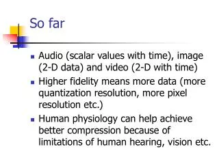
So far. Audio (scalar values with time), image (2-D data) and video (2-D with time) Higher fidelity means more data (more quantization resolution, more pixel resolution etc.) Human physiology can help achieve better compression because of limitations of human hearing, vision etc.

So far
E N D
Presentation Transcript
So far • Audio (scalar values with time), image (2-D data) and video (2-D with time) • Higher fidelity means more data (more quantization resolution, more pixel resolution etc.) • Human physiology can help achieve better compression because of limitations of human hearing, vision etc. • Next, we focus deeply into compression techniques • You will find that higher fidelity might actually compress better than lower fidelity (e.g., 8 bit photo vs 24 bit photo)
Lossless compression •Compression: the process of coding that will effectively reduce the total number of bits needed to represent certain information. If the compression and decompression processes induce no information loss, then the compression scheme is lossless; otherwise, it is lossy. Compression ratio:
Shannon’s theory The entropyη of an information source with alphabet S = {s1, s2, . . . , sn} is: (7.3) pi – probability that symbol si will occur in S. Compression is not possible for a) because entropy is 8 (need 8 bits per value)
Run length coding Memoryless Source: an information source that is independently distributed. Namely, the value of the current symbol does not depend on the values of the previously appeared symbols Rationale for RLC: if the information source has the property that symbols tend to form continuous groups, then such symbol and the length of the group can be coded.
Variable length codes • Different length for each symbol • Use occurence frequency to choose lengths • An Example: Frequency count of the symbols in ”HELLO”.
Huffman Coding • Initialization: Put all symbols on a list sorted according to their frequency counts • Repeat until the list has only one symbol left: • From the list pick two symbols with the lowest frequency counts. Form a Huffman sub-tree that has these two symbols as child nodes and create a parent node • Assign the sum of the children’s frequency counts to the parent and insert it into the list such that the order is maintained • Delete the children from the list • Assign a codeword for each leaf based on the path from the root.
Fig. 7.5: Coding Tree for “HELLO” using the Huffman Algorithm.
Huffman Coding (cont’d) • new symbols P1, P2, P3 are created to refer to the parent nodes in the Huffman coding tree • After initialization: L H E O • After iteration (a): L P1 H • After iteration (b): L P2 • After iteration (c): P3
Properties of Huffman Coding • Unique Prefix Property: No Huffman code is a prefix of any other Huffman code - precludes any ambiguity in decoding • Optimality: minimum redundancy code - proved optimal for a given data model (i.e., a given, accurate, probability distribution): • The two least frequent symbols will have the same length for their Huffman codes, differing only at the last bit • Symbols that occur more frequently will have shorter Huffman codes than symbols that occur less frequently • The average code length for an information source S is strictly less than η + 1
Adaptive Huffman Coding Extended Huffman is in book: group symbols together Adaptive Huffman: statistics are gathered and updated dynamically as the data stream arrives
Adaptive Huffman Coding (Cont’d) • Initial_code assigns symbols with some initially agreed upon codes, without any prior knowledge of the frequency counts. • update_tree constructs an Adaptive Huffman tree. It basically does two things: • increments the frequency counts for the symbols (including any new ones) • updates the configuration of the tree. • The encoder and decoder must use exactly the same initial_code and update_tree routines
Notes on Adaptive Huffman Tree Updating The tree must always maintain its sibling property, i.e., all nodes (internal and leaf) are arranged in the order of increasing counts If the sibling property is about to be violated, a swap procedure is invoked to update the tree by rearranging the nodes When a swap is necessary, the farthest node with count N is swapped with the node whose count has just been increased to N +1
Fig. 7.6: Node Swapping for Updating an Adaptive Huffman Tree
• It is important to emphasize that the code for a particular symbol changes during the adaptive Huffman coding process. For example, after AADCCDD, when the character D overtakes A as the most frequent symbol, its code changes from 101 to 0 Table 7.4 Sequence of symbols and codes sent to the decoder
7.5 Dictionary-based Coding • LZW uses fixed-length code words to represent variable-length strings of symbols/characters that commonly occur together, e.g., words in English text • LZW encoder and decoder build up the same dictionary dynamically while receiving the data • LZW places longer and longer repeated entries into a dictionary, and then emits the code for an element, rather than the string itself, if the element has already been placed in the dictionary
LZW compression for string “ABABBABCABABBA” The output codes are: 1 2 4 5 2 3 4 6 1. Instead of sending 14 characters, only 9 codes need to be sent (compression ratio = 14/9 = 1.56).
LZW decompression (1 2 4 5 2 3 4 6 1) ABABBABCABABBA
LZW Coding (cont’d) In real applications, the code length l is kept in the range of [l0, lmax]. The dictionary initially has a size of 2l0. When it is filled up, the code length will be increased by 1; this is allowed to repeat until l = lmax When lmaxis reached and the dictionary is filled up, it needs to be flushed (as in Unix compress, or to have the LRU (least recently used) entries removed
7.6 Arithmetic Coding • Arithmetic coding is a more modern coding method that usually out-performs Huffman coding • Huffman coding assigns each symbol a codeword which has an integral bit length. Arithmetic coding can treat the whole message as one unit • More details in the book
7.7 Lossless Image Compression Due to spatial redundancy in normal images I, the difference image d will have a narrower histogram and hence a smaller entropy
Lossless JPEG • A special case of the JPEG image compression • The Predictive method • Forming a differential prediction: A predictor combines the values of up to three neighboring pixels as the predicted value for the current pixel
2. Encoding: The encoder compares the prediction with the actual pixel value at the position ‘X’ and encodes the difference using Huffman coding