Land Use Patterns in Central Platte River Basin: A Comprehensive Study Using Landsat Imagery
310 likes | 433 Views
This study outlines the methodology for delineating land use patterns in the Central Platte River Basin using Landsat Thematic Mapper imagery from 1997. It includes the acquisition of 24 images across various seasons, image processing techniques to mask out unwanted elements, and detailed image classification through supervised and unsupervised methods. The objective is to categorize land cover into distinct classes utilizing spectral patterns from satellite data. The research incorporates data collected from the Farm Service Agency to enhance accuracy and aims to support hydrological studies in the region.

Land Use Patterns in Central Platte River Basin: A Comprehensive Study Using Landsat Imagery
E N D
Presentation Transcript
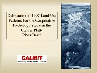
Delineation of 1997 Land Use Patterns For the Cooperative Hydrology Study in the Central PlatteRiver Basin
Methodology • Acquire Landsat Thematic Mapper Imagery • 10 Path/Row scenes, the majority of which having three dates (spring, summer, and fall) – total of 24 images
Methodology • Image Processing • Register to a common map projection • Mask out urban areas, clouds, cloud shadows, and jet contrails • Subset bands 2-5, and 7 from each date of imagery • Layer stack remaining 5 bands from each scene to create one 15-band image for each Path/Row with three dates of imagery.
Spectral Band Spectral Range (m) Nominal Spectral Location Ground Resolution (m) 1 0.45- 0.52 Visible Blue 30 2 0.52 – 0.60 Visible Green 30 3 0.63 – 0.69 Visible Red 30 4 0.76 – 0.90 Near infrared 30 5 1.55 – 1.75 Mid-infrared 30 6 10.4 – 12.5 Thermal infrared 120 7 2.08 – 2.35 Mid-infrared 30 Methodology Characteristics of Landsat 5
Methodology • Image Classification • Primary objective is to automatically categorize all pixels in an image into land cover classes • It is the spectral pattern present within the data for each pixel that is used as the numerical basis for the classification
6 COHYST 26 Output Classes
Supervised Classification • The user identifies pixels in the imagery which represent sites of known land cover • Identifying these areas in the satellite imagery you can train the computer system to identify pixels with similar spectral characteristics • Spectral signatures are collected at the training sites • Signatures are used as various types of land cover can be recognized and distinguished from each other by differences in relative reflectances
Spectral Reflectance Curves Spectral Reflectance Values ----- May ------ ----- August ----- --- September ---- TM Image Bands 2, 3, 4, 5, and 7 for 3 dates of imagery
Data used in collecting signatures • Crop information gathered from Farm Service Agency reporting records for 1997 • Records were randomly divided, half used for collecting signatures and half used for accuracy assessment • DOQQ’s- were used to locate forest, roads and non-Ag. Features (farmsteads, feedlots)
Wetland Type Wetland Code Water Regime Emergent PEM Permanently Flooded Pond with floating or submerged aquatic vegetation PAB Intermittently Exposed Pond with open water PUB Semi-permanently flooded Data used in collecting signatures National Wetlands Inventory (NWI) – signatures were collected from wetlands greater than 3X3 pixels or 90X90 meters square in size from the following types:
Class Name Scene 29/31 29/32 30/32 31/31 31/32 32/31 33/31 Corn 43 132 343 70 201 75 130 Sugar Beets 3 7 33 Soybeans 21 46 80 3 14 9 64 Sorghum 29 54 5 2 2 2 Dry Edible Beans 9 4 7 Potatoes 3 1 1 Alfalfa 12 14 55 31 45 6 38 Small Grains 1 38 101 21 220 188 230 Range/pasture 25 55 130 99 239 150 128 Open Water 6 3 35 63 112 230 31 Forest/woodlands 8 18 19 89 121 72 20 Wetlands 86 163 90 217 118 127 107 Other Ag. lands 6 11 17 13 5 2 28 Sunflower 2 3 2 Summer fallow 8 46 16 209 136 161 Roads 3 4 5 19 7 5 2 Number of Spectral Signatures for usedfor Each Land Cover Class by Scene • Numbers reflect the size of the scene, diversity and acreage of crops in that scene, and data available from FSA records
Supervised Classification Example Original Imagery Classified Image TM bands (4, 3, 2)
After the Initial Classification • Spectral signatures were evaluated / Areas of mixed pixels identified • Mixed pixels were reclassified using a ‘cluster busting’ technique • Mixed pixels were identified and masked from the raw TM data and then re-classified using an unsupervised classification approach • The output clusters where re-assigned to the classes they most closely resembled.
Unsupervised Classification • Was run on scenes where less than three dates of imagery were available and on clouded areas • Unsupervised classification does not use training sites • The image is classified using mathematical algorithms that search for natural groups of the spectral properties of pixels • Output clusters identified based on surrounding areas of overlap with the supervised classification • Clusters were also identified using FSA reporting records used to identify training sites
Classified triple date scenes Classified double date scenes Classified single date scenes Bottom Classified cloud covered areas Combining of Map Layers • After final edits were made to the classified imagery, all separate layers were combined to produce a single classified image Mosaic Order of Classified Scenes Top • When scenes were mosaiced, urban polygon areas were laid back • into the imagery
Delineation of Irrigated Areas • Center Pivots on screen digitized using satellite imagery • Irrigation data obtained from: • Pathfinder Irrigation District • Central Nebraska Pubic Power District • Paper irrigation rights maps from Department of Natural resources – Digitized • All irrigation data were printed on maps divided by Natural Resource District and then sent out to each NRD and checked for accuracy • When maps were returned the original vector files were edited and then all files were merged into one final vector irrigation map
Irrigation Analysis • Irrigation vector data were rasterized so that it could be combined with the classified imagery • The two grids were compared and a new grid was created using the DOCELL command within ArcInfo GRID + Irrigation Map Classified Image Irrigation.aml New Classified Image With Irrigated and Dryland Crops Identified
Land Use Classification Example Legend Corn Sugar Beets Soybeans Sorghum (Milo) Dry Edible Beans Potatoes Alfalfa Small Grains Range/Pasture/Grass Urban Open Water Riparian Forests/Woodlands Wetlands Other Ag. Lands Sunflower Summer Fallow Roads (Outline) Irrigated Areas
Accuracy Assessment • Reference data were collected from the FSA records set aside for the accuracy assessment • Random points were generated across the study area • Digital section boundaries were used to clip out the random points that fell into those sections for which we had reference data • These points were then labeled based on the FSA data • 100 reference points were used for each selected land cover class, a total of 1900 reference points were used in the final accuracy assessment
Accuracy Assessment • Error Matrix • Cross tabulation of classes assigned in the classified image versus the observed reference data • Used to determine producer’s, user’s, and overall accuracy • Producer’s Accuracy • Number correctly classified / Number of reference points • User’s Accuracy • Number correctly classified / Total number classified • Overall Accuracy • Average of Producer’s and User’s Accuracy
Accuracy Assessment Accuracy Totals for Crops Without Irrigation Layer
Accuracy Assessment • KAPPA Analysis • Measures the difference between the actual agreement between the reference data and an automated classifier and the chance agreement between the reference data and a random classifier • Yields a KHAT statistic • Values range from 0.0 –1.0 • 0.0 indicating agreement no greater than expect by chance alone • 1.0 indicating a perfect agreement • KHAT statistic for the classification = .7736
Accuracy Assessment • Weighted KAPPA • Using KAPPA to derive the KHAT statistic is suitable when all the error in the matrix can be considered of equal importance • For the COHYST study not all land cover classes have the same influence • Assigning weights for the weighted KAPPA were based on acreage totals by land cover class.
Accuracy Assessment • Weighted KAPPA • Relative weights were assigned to each cell in the error matrix and weighted KAPPA was computed for the entire image • The weighted Kappa produced a KHAT statistic of .7940 compared to the original KHAT statistic of .7736
Causes of Lower Accuracies and Sources of Error • Farm Service Agency Reporting Records • While they were the best available choice for ground truth on crop types, inaccuracies still existed in the data to select signatures and determine accuracy • Field boundaries were not always correctly defined • Aerial phototgraphy on which the FSA records were based was sometimes out of date • Due to the random selection of sections, not all crops may have been represented or there may have been minimal number of signatures • This was the case for crops such as dry edible beans, sugar beets, potatoes, and sunflowers.
Causes of Lower Accuracies and Sources of Error • Error was also introduced in determining irrigated areas • Not all counties labeled crops as irrigated or non-irrigated on the FSA reporting records • Since the FSA data formed the basis for the accuracy assessment, mislabeling errors were most likely encountered • Irrigation records were not always available for 1997 • Some counties only had records of irrigation if the acres were certified for crop insurance