In Chapter 4, you will learn:

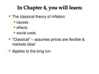
1. In Chapter 4, you will learn: The classical theory of inflation causes effects social costs “Classical” – assumes prices are flexible & markets clear Applies to the long run

2. The connection between money and prices • Inflation rate = the percentage increase in the average level of prices = ∆P/P • Price = amount of money required to buy a good. • Because prices are defined in terms of money, we need to consider the nature of money, the supply of money, and how it is controlled.

3. Money: Definition Money is the stock of assets that can be readily used to make transactions.

4. Money: Functions • medium of exchangewe use it to buy stuff • store of valuetransfers purchasing power from the present to the future • unit of accountthe common unit by which everyone measures prices and values

5. Money: Types 1. Fiat money • has no intrinsic value • example: the paper currency we use 2. Commodity money • has intrinsic value • example: gold coins,

6. The money supply and monetary policy definitions • The money supply is the quantity of money available in the economy. • Monetary policy is the control over the money supply.

7. The central bank • Monetary policy is conducted by a country’s central bank. • In the U.S., the central bank is called the Federal Reserve (“the Fed”).

8. C Currency $850 M1 C + demand deposits, travelers’ checks, other checkable deposits $1596 M2 M1 + small time deposits, savings deposits, money market mutual funds, money market deposit accounts $8328 Money supply measures, May 2009 symbol assets included amount ($ billions)

9. The Quantity Theory of Money • A simple theory linking the inflation rate to the growth rate of the money supply. • Begins with the concept of velocity…

10. Velocity • basic concept: the rate at which money circulates • definition: the number of times the average dollar bill changes hands in a given time period • example: • $500 billion in transactions • money supply = $100 billion • Each dollar is used on average in five transactions. • So, velocity = 5

11. Velocity, cont. • This suggests the following definition: where V = velocity T = value of all transactions M = money supply

12. Velocity, cont. • Use nominal GDP as a proxy for total transactions: Then, where P = price of output (GDP deflator) Y = quantity of output (real GDP) P Y = value of output (nominal GDP)

13. The quantity equation (equation of exchange) • The quantity equation (equation of exchange) M V = P Y follows from the preceding definition of velocity. • It is an identity:it holds by definition of the variables.

14. Money demand and the quantity equation • M/P = real money balances, the purchasing power of the money supply. • A simple money demand function: (M/P)d = kYwherek = how much money people wish to hold for each dollar of income. (kis exogenous)

15. Money demand and the quantity equation • money demand: (M/P)d = kY • quantity equation: M V = P Y • The connection between them: k = 1/V • When people hold lots of money relative to their incomes (kis large), money changes hands infrequently (Vis small).

16. The quantity theory of money • starts with quantity equation (equation of exchange • assumes V is constant & exogenous: Then, quantity equation becomes: This is the Quantity Theory of Money

17. The quantity theory of money How the price level is determined: • With V constant, the money supply determines nominal GDP (P Y ). • Real GDP (Y) is determined by the economy’s supplies of K and L and the production function (Chap 3). • The price level is P = (nominal GDP)/(real GDP).

18. The quantity theory of money • Recall from Chapter 2: The growth rate of a product equals the sum of the growth rates. • The quantity equation in growth rates:

19. The quantity theory of money  (Greek letter “pi”) denotes the inflation rate: The result from the preceding slide: Solve this result for :

20. The quantity theory of money • Normal economic growth requires a certain amount of money supply growth to facilitate the growth in transactions. • Money growth in excess of this amount leads to inflation.

21. The quantity theory of money Y/Y depends on growth in the factors of production and on technological progress (all of which we take as given, for now). Hence, the Quantity Theory predicts a one-for-one relation between changes in the money growth rate and changes in the inflation rate.

22. The Quantity Theory and the data The quantity theory of money implies: 1. Countries with higher money growth rates should have higher inflation rates. 2. The long-run trend behavior of a country’s inflation should be similar to the long-run trend in the country’s money growth rate. Are the data consistent with these implications?

23. International data on inflation and money growth Belarus Indonesia Inflation rate (percent, logarithmic scale) Turkey Ecuador Argentina Singapore Money supply growth(percent, logarithmic scale)

24. Seigniorage • To spend more without raising taxes or selling bonds, the govt can print money. • The “revenue” raised from printing money is called seigniorage (pronounced SEEN-your-idge). • The inflation tax:Printing money to raise revenue causes inflation. Inflation is like a tax on people who hold money.

25. Inflation and interest rates • Nominal interest rate, inot adjusted for inflation • Real interest rate, radjusted for inflation:r = i 

26. The Fisher effect • The Fisher equation:i = r +  • Chap 3: S = I determines r.(S, I and r are real variables) • Hence, an increase in  causes an equal increase in i. • This one-for-one relationship is called the Fisher effect.

27. U.S. inflation and nominal interest rates, 1960-2009 nominal interest rate inflation rate

28. Inflation and nominal interest rates across countries (1999 – 2007) Nominal interest rate(percent, logarithmic scale) Romania Georgia Zimbabwe Turkey Brazil Israel Kenya U.S. Ethiopia Germany Inflation rate(percent, logarithmic scale)

29. NOW YOU TRY: Applying the theory Suppose V is constant, Mis growing 5% per year, Y is growing 2% per year, and r= 4. a. Solve for i. b. If the Fed increases the money growth rate by 2 percentage points per year, find i. c. Suppose the growth rate of Y falls to 1% per year. What will happen to ? What must the Fed do if it wishes to keep constant?

30. Two real interest rates FIRST - Notation (7th Edition): •  = actual inflation rate (not known until after it has occurred) • E = expected inflation rate Two real interest rates: • i – E = ex ante real interest rate: the real interest rate people expect at the time they buy a bond or take out a loan • i –  = ex postreal interest rate:the real interest rate actually realized

31. Two real interest rates Notation (earlier Editions):  = actual inflation rate (not known until after it has occurred) e = expected inflation rate Two real interest rates: i – e = ex ante real interest rate: the real interest rate people expect at the time they buy a bond or take out a loan i –  = ex postreal interest rate:the real interest rate actually realized

32. Money demand and the nominal interest rate • In the Quantity Theory of Money, the demand for real money balances depends only on real income Y. • Another determinant of money demand: the nominal interest rate, i. • the opportunity cost of holding money (instead of bonds or other interest-earning assets). • Hence, i   in money demand.

33. (M/P)d = real money demand, depends: negatively on i i is the opportunity cost of holding money positively on Y higher Y more spending  so, need more money (“L” is used for the money demand function because money is the most liquid asset.) The money demand function

34. When people are deciding whether to hold money or bonds, they don’t know what inflation will turn out to be. Hence, the nominal interest rate relevant for money demand is r + E. The money demand function

35. The supply of real money balances Real money demand Equilibrium

36. variable how determined (in the long run) M exogenous (the Fed) r adjusts to ensure S = I (Chap. 3) Y (Chap. 3) P adjusts to ensure What determines what

37. How P responds to M • For given values of r, Y, and E , a change in Mcauses P to change by the same percentage – just like in the quantity theory of money.

38. What about expected inflation? • Over the long run, people don’t consistently over- or under-forecast inflation, so E =  on average (e =  on average). • In the short run, e may change when people get new information. • EX: Fed announces it will increase Mnext year. People will expect next year’s P to be higher, so E rises. • This affects P now, even though M hasn’t changed yet….

39. How P responds to E • For given values of r, Y, and M , Remember: M x V = P x Y

40. A common misperception • Common misperception: inflation reduces real wages • This is true only in the short run, when nominal wages are fixed by contracts. • (Chap. 3) In the long run, the real wage is determined by labor supply and the marginal product of labor, not the price level or inflation rate. • Consider the data…

41. The CPI and Average Hourly Earnings, 1965-2009 900 $20 800 Real average hourly earnings in 2009 dollars, right scale 700 $15 600 500 1965 = 100 Hourly wage in May 2009 dollars $10 400 Nominal average hourly earnings, (1965 = 100) 300 $5 200 CPI (1965 = 100) 100 0 $0 1965 1970 1975 1980 1985 1990 1995 2000 2005 2010

42. Labor productivity and wages Theory: Real wages depend on labor productivity U.S. data:

43. The classical view of inflation • The classical view: A change in the price level is merely a change in the units of measurement. Then, why is inflation a social problem?

44. The social costs of inflation …fall into two categories: 1. costs when inflation is expected 2. costs when inflation is different than people had expected

45. The costs of expected inflation: 1. Shoeleather cost • def: the costs and inconveniences of reducing money balances to avoid the inflation tax. •   i   real money balances • Remember: In long run, inflation does not affect real income or real spending. • So, same monthly spending but lower average money holdings means more frequent trips to the bank to withdraw smaller amounts of cash.

46. The costs of expected inflation: 2. Menu costs • def: The costs of changing prices. • Examples: • cost of printing new menus • cost of printing & mailing new catalogs • The higher is inflation, the more frequently firms must change their prices and incur these costs.

47. The costs of expected inflation: 3. Relative price distortions • Firms facing menu costs change prices infrequently. • Example: A firm issues new catalog each January. As the general price level rises throughout the year, the firm’s relative price will fall. • Different firms change their prices at different times, leading to relative price distortions… …causing microeconomic inefficiencies in the allocation of resources.

48. The costs of expected inflation: 4. Unfair tax treatment Some taxes are not adjusted to account for inflation, such as the capital gains tax. Example: • Jan 1: you buy $10,000 worth of IBM stock • Dec 31: you sell the stock for $11,000, so your nominal capital gain is $1000 (10%). • Suppose  = 10% during the year. Your real capital gain is $0. • But the govt requires you to pay taxes on your $1000 nominal gain!!

49. The costs of expected inflation: 5. General inconvenience • Inflation makes it harder to compare nominal values from different time periods. • This complicates long-range financial planning.

50. Additional cost of unexpected inflation: Arbitrary redistribution of purchasing power • Many long-term contracts not indexed, but based on E. • If turns out different from E, then some gain at others’ expense. Example: borrowers & lenders • If  > E, then (i ) < (iE) and purchasing power is transferred from lenders to borrowers. • If  < E, then purchasing power is transferred from borrowers to lenders.