Download
1 / 50
530 likes | 802 Views
Chapter 2 Discrete System Analysis – Discrete Signals. Continuous-time analog signal. Sampling of Continuous-time Signals. sampler. Output of sampler. T. How to treat the sampling process mathematically ?.

E N D
Continuous-time analog signal Sampling of Continuous-time Signals sampler Output of sampler T How to treat the sampling process mathematically ? For convenience, uniform-rate sampler(1/T) with finite sampling duration (p) is assumed. p 1 time T where p(t) is a carrier signal (unit pulse train)
carrier signal p(t) PAM This procedure is called a pulse amplitude modulation (PAM) The unit pulse train is written as By Fourier series or magnitude phase
-4s -3s -2s -s 0 s 2s 3s 4s
|F(j)| 1 c : Cutoff frequency -s /2 -c 0 c s/2
0 s -s frequency folding 0 -s s
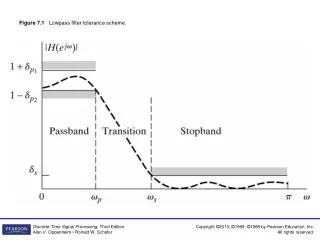
Theorem : Shannon’s Sampling Theorem To recover a signal from its sampling, you must sample at least twice the highest frequency in the signal. Remarks: i) A practical difficulty is that real signals do not have Fourier transforms that vanish outside a given frequency band. To avoid the frequency folding (aliasing) problem, it is necessary to filter the analog signal before sampling. Note: Claude Shannon (1917 - 2001)
ii) Many controlled systems have low-pass filter characteristics. iii) Sampling rates > 10 ~ 30 times of the BW of the system. iv) For the train of unit impulses -2s -s s 0
|X(j)| |X*(j)| |Y(j)| Ideal filterG(j) 1 1/T 1/T -c 0 c -c 0 c -c 0 c reconstruction Remarks : • Impulse response of ideal low-pass filter (non-causality) • Ideal low-pass filter is not realizable in a physical system. • How to realize it in a physical system ? ZOH or FOH T sampling
ii)(Aliasing) It is not possible to reconstruct exactly a continuous-time signal in a practical control system once it is sampled.
iii)(Hidden oscillation) If the continuous-time signal involves a frequency component equal to n times the sampling frequency (where n is an integer), then that component may not appear in the sampled signal.
Signal Reconstruction How to reconstruct (approximate) the original signal from the sampled signal? -ZOH (zero-order hold) - FOH (first-order hold)
ZOH (Zero-order Hold) zero-order hold reconstruction k-1 k k+1 time T
Remarks: i) The ZOH behaves essentially as a low-pass filter. ii) The accuracy of the ZOH as an extrapolator depends greatly on the sampling frequency, . • iii) In general, the filtering property of the ZOH is used almost • exclusively in practice.
k-1 k k+1 T FOH (First-order Hold)
2 1 0 T 2T 3T time -1
first zero zero first Large lag(delay) in high frequency makes a system unstable
Remark: • At low frequencies, the phase lag produced by the ZOH exceeds that of FOH, but as the frequencies become higher, the opposite is true
T Z-transform
Because R(z) is a power series in z-1 , the theory of power series may be applied to determine the convergence of • the z-transform. ii) The series in z-1 has a radius of convergence such that the series converges absolutely when | z-1 |< iii) If 0, the sequence {rk} is said to be z-transformable.
Remark: unit impulse = Z-transform of Elementary Functions i) Unit pulse function ii) Unit step function
iv) Polynomial function v) Exponential function
Remark: Refer Table 2-1 in pp.29-30 (Ogata) Also, refer Appendix B.2 Table in pp. 702-703(Franklin)
Correspondence with Continuous Signals z=esT s-plane z-plane
② ③ ① -1 0 1 ⑤ ④ ImZ ImZ 0 1 ReZ ReZ j ③ ② ① 0 ④ ⑤ j -2 1 0
ImZ ImZ 1 ReZ ReZ j 0 0 fixed j 0
Important Properties and Theorems of the z-transform 1. Linearity 2. Time Shifting
3. Convolution 4. Scaling 5. Initial Value Theorem
Remark: Refer Table 2-2 in p. 38.(Ogata) Also, refer Appendix B.1 Table in p.701(Franklin)
Discrete-time domain Continuous-time domain S-plane Z-plane
Inverse z-transform • Power Series Method (Direct Division) • ii) Computational Method : • - MATLAB Approach - Difference Equation Approach • iii) Partial Fraction Expansion Method • iv) Inversion Integral Method
Example 4) Inverse Integral Method : where cis a circle with its center at the origin of the z plane such that all poles of F(z)zk-1 are inside it.
Case 1) simple pole Case 2) m multiple poles