A Brief Introduction to Antennas & Transmission Lines Prof. John Vesecky

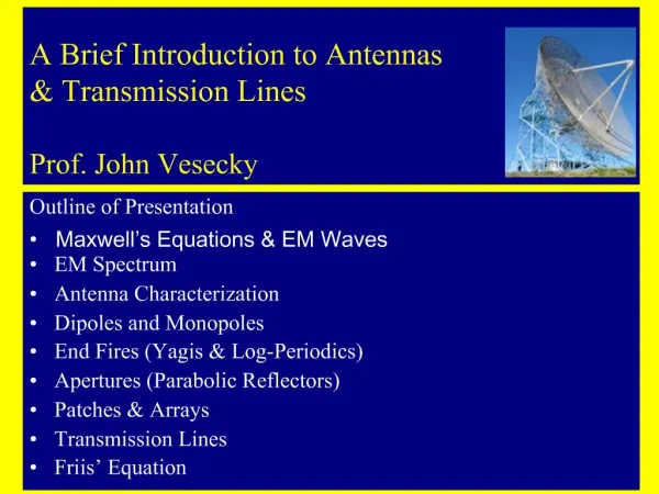
1. Outline of Presentation • Maxwell’s Equations & EM Waves EM Spectrum Antenna Characterization Dipoles and Monopoles End Fires (Yagis & Log-Periodics) Apertures (Parabolic Reflectors) Patches & Arrays Transmission Lines Friis’ Equation A Brief Introduction to Antennas& Transmission LinesProf. John Vesecky

2. I. Outline for Wire, Aperture and Patch Antennas • EM Spectrum • Antenna Characterization • Dipoles and Monopoles • End Fires (Yagis & Log-Periodics) • Apertures (Parabolic Reflectors) • Patches & Arrays

3. • v2 = 1/(oµo) so v = 3 x 108 m/s o = 8.855 x 10-12 Farads/m µo = 1.2566 x 10-6 Henrys/m EM waves in free space propagate freely without attenuation What is a plane wave? Example is a wave propagating along the x-direction Fields are constant in y and z directions, but vary with time and space along the x-direction Most propagating radio (EM) waves can be thought of a plane waves on the scale of the receiving antenna EM waves in free space

4. E & H fields and Poynting Vector for Power Flow • Power flow in the EM field • P = E x H (P is Poynting vector) • In free space E and H are perpendicular • P is perpendicular to both E and H • Plane wave radiated by an antenna • P = E x H -> Eo Ho Sin2(t-kx) • P = [Eo2/] Sin2(t-kx) • Pavg = (1/2) [Eo2/] in W/m2 •  = impedance of free space = 377 

5. Electromagnetic Spectrum After Kraus & Marhefka, 2003

6. Frequencies & Wavelengths After Kraus & Marhefka, 2003

7. RF Bands, Names & Users After Kraus & Marhefka, 2003

8. Radiation from a Short Antenna Element or Hertzian Dipole • Using the Electrodynamic Retarded Potential A (Vector) we can derive (see Ramo et al., 1965 or Skilling, 1948, Ulaby, 2007 or any EM theory book) E and H fields associated with a small element of current of length l (<< ) that has the current varying as i = I Sin (t) • This could be a wire or charge moving in space, e.g. in the plasma of the ionosphere or a star or nebula • E and H fields at r could be in the r,  or  directions

9. Radiation from a Short Antenna Element or Hertzian Dipole A(r) = (µo/4) (e-jkr/r)∫V [J (e-jkr’/r’)] dv’ H = (1/µo) curl A • H = (Io l k2/4) e-jkr [j/(kr) + 1/(kr)2] sin  • Hr = 0 and H = 0 E = (1/jo) curl H • Er = (2Io l k2/4) o e-jkr [1/(kr)2 - j/(kr)3] • E = (Io l k2/4) o e-jkr [j/kr + 1/(kr)2 - j/(kr)3] o = Sqrt(µo/o) = 377 Ω

10. Radiation from a Short Antenna Element • Terms that fall off as 1/r3 or 1/r2 are small at any significant distance from an antenna • Remaining “radiation” terms fall off only as 1/r and thus transmit energy for long distances also E and H fields are in phase • When one is in the “near field” the 1/r3 or 1/r2 the other terms are important

11. Antenna Field Zones • The dividing line “Rule of Thumb” is R = 2L2/ • The near field or Fresnel zone is r < R • The far field or Fraunhofer zone is r > R

12. Intuitive Picture of Radiation

13. Intuitive Picture of Radiation

14. Polarization of EM Waves AR = Axial Ratio

15. Simple Dipole Antenna

16. Antenna Characterization •Directivity • Power Pattern • Antenna Gain • Effective Area • Antenna Efficiency

17. Antenna Directivity • An omnidirectional antenna radiates power into all directions (4 steradians) equally • Typically an antenna wants to beam radiation in a particular direction • Directivity D = 4/,  is the antenna beam solid angle • What  would be for one octant (x,y,z all > 0) ?

18. Normalized Antenna Power Pattern • Pn(, ) = S()/S()max • S() = Poynting vector magnitude = [E2 + E2]/ •  = 376.7 free space) After Kraus (2003)

19. Antenna Gain • Gain is like directivity, but includes losses as well • G() ≈ /() is nondimensional° --  accounts for losses • dB = 10 log(x/xref) -- always refers to power • Gain for Typical Antenna with significant directivity • G() ≈ 2500/(° °), taking into account beam shape and typical losses

20. Estimating Effective Antenna Area & Gain • Definition: G = (4 Ae)/2 • Ae =  A, where A is the physical area and  is the antenna efficiency • To get the average power available at the antenna terminals we use • Pav,Ant = Pav,Poynting (Average Poynting Flux) Ae • A crude estimate of G can be obtained by letting •  ≈ (/d), where d is the antenna dimension along the direction of the angle  -- big antenna means small  • and G() ≈ /()

21. Radiation Resistance & Antenna Efficiency • Radiation resistance (Rrad) is a fictitious resistance, such that the average power flow out of the antenna is Pav = (1/2) <I>2 Rrad • Using the equations for our short (Hertzian) dipole we find that Rrad = 80 2 (l/)2 ohms • Antenna Efficiency  = Rrad/(Rrad+ Rloss) where Rloss = ohmic losses as heat • Gain = x Directivity --- G = D

22. Antenna Family

23. Short Dipole Antenna Analysis • Consider a finite, but short antenna with l << situated in free space • Current is charging the uniformly distributed capacitance of the antenna wire & so has a maximum at the middle and tapers toward zero at the ends • Each element dl radiates per our radiation equations (previous slide), namely • In the far field E = ( I dl sin/(2 r )) cos {[t-(r/c)]} • The  direction is in the same plane as the element dl and the radial line from antenna center to observer and perpendicular to r

24. Short Dipole Antenna Result • The resultant field at the observer at r is the sum of the contributions from the elemental lengths dl • Each contribution is essentially the same except that the current I varies • Radiation contribution to the sum is strongest from the center and weakest at the ends • This can be summarized as the rms field strength in volts per meter as E,rms = [ Io le sin/(2 r )] -- V/m • What do you think the effective length le & current Io are? • The radiated power is Pav = (E,rms)2/(2

25. Modifications for Half Wavelength Dipole • For antennas comparable in size to  • Current distribution is not linear • Phase difference between different parts of the antenna • Current distribution on /2 dipole • Antenna acts like open circuit transmission line with uniformly distributed capacitance • Sinusoidal current distribution results

26. Fields from /2 Dipole • To take account of the phase differences of the contributions from all the elements dl we need to integrate over the entire length of the antenna as shown by the figure (from Skilling, 1948) E = ∫±/4 ( Io sine/2 re) cos kx cos [t-(re/c)] dx • Integral is from -/4 to /4, i.e. over the antenna length • Result of integration E = (Io/2r) cos [t-(r/c)] {cos [( /2) cos] / sin} • We know that Er = E= 0 as for the Hertzian dipole

27. /2 and  Dipole Antenna Pattern (E-field)

28. Monopole over a Conducting Plane -- /4 Vertical

29. /4 Vertical over Ground Plane & Real Earth • Solid line is for perfectly conducting Earth • Shaded pattern shows how the pattern is modified by a more realistic Earth with dielectric constant k = 13 and conductivity G = 0.005 S/m

30. Yagi - Uda • Driven element induces currents in parasitic elements • When a parasitic element is slightly longer than /2, the element acts inductively and thus as a reflector -- current phased to reinforce radiation in the maximum direction and cancel in the opposite direction • The director element is slightly shorter than/2, the element acts inductively and thus as a director -- current phased to reinforce radiation in the maximum direction and cancel in the opposite direction • The elements are separated by ≈ 0.25

31. 3 ElementYagi Antenna Pattern

32. 2.4 GHz Yagi with 15dBi Gain • G ≈ 1.66 * N (not dB) • N = number of elements • G ≈ 1.66 *3 = 5 = 7 dB • G ≈ 1.66 * 16 = 27 = 16 dB

33. Log-Periodic Antennas • A log periodic is an extension of the Yagi idea to a broad-band, perhaps 4 x in wavelength, antenna with a gain of ≈ 8 dB • Log periodics are typically used in the HF to UHF bands

34. Parabolic Reflectors • A parabolic reflector operates much the same way a reflecting telescope does • Reflections of rays from the feed point all contribute in phase to a plane wave leaving the antenna along the antenna bore sight (axis) • Typically used at UHF and higher frequencies

35. Stanford’s Big Dish • 150 ft diameter dish on alt-azimuth mount made from parts of naval gun turrets • Gain ≈ 4 A/2≈ 2 x 105 ≈ 53 dB for S-band (l ≈15 cm)

36. Patch Antennas • Radiation is from two “slots” on left and right edges of patch where slot is region between patch and ground plane • Length d = /r1/2 Thickness typically ≈ 0.01  • The big advantage is conformal, i.e. flat, shape and low weight • Disadvantages: Low gain, Narrow bandwidth (overcome by fancy shapes and other heroic efforts), Becomes hard to feed when complex, e.g. for wide band operation After Kraus & Marhefka, 2003

37. Patch Antenna Pattern

38. Array Antennas

39. Patch Antenna Array for Space Craft • The antenna is composed of two planar arrays, one for L-band and one for C-band. • Each array is composed of a uniform grid of dual-polarized microstrip antenna radiators, with each polarization port fed by a separate corporate feed network. • The overall size of the SIR-C antenna is 12.0 x 3.7 meters • Used for synthetic aperture radar

40. Very Large Array Organization: National Radio Astronomy Observatory Location:Socorro NM Wavelength: radio 7 mm and larger Number & Diameter 27 x 25 m Angular resolution: 0.05 (7mm) to 700 arcsec http://www.vla.nrao.edu/

41. Radio Telescope Results • This is a false-color image of the radio galaxy 3C296, associated with the elliptical galaxy NGC5532. Blue colors show the distribution of stars, made from an image from the Digitized Second Palomar Sky Survey, and red colors show the radio radiation as imaged by the VLA, measured at a wavelength of 20cm. Several other galaxies are seen in this image, but are not directly related to the radio source. The radio emission is from relativistic streams of high energy particles generated by the radio source in the center of the radio galaxy. Astronomers believe that the jets are fueled by material accreting onto a super-massive black hole. The high energy particles are confined to remarkably well collimated jets, and are shot into extragalactic space at speeds approaching the speed of light, where they eventually balloon into massive radio lobes. The plumes in 3C296 measure 150 kpc or 480,000 light years edge-to-edge diameter (for a Hubble constant of 100 km/s/Mpc). • Investigator(s):ﾊ J.P. Leahy & R.A. Perley. Optical/Radio superposition by Alan Bridle

42. Impedance Matching • SWR = (1 + ||)/ (1 - ||)

43. Pr = Pt {(Aet Aer)/(2 r2)} S/N = Signal to noise ratio = Pr/(kTsysB) where Tsys = system noise temperature, typically 10’s to 1000’s of K depending on receiver characteristics k = 1.38 x 10-23 J/K B = bandwidth in Hz Friis’ Transmission Formula

44. References 1 • Balanis, C.A., Antenna Theory, Analysis and Design, 2nd ed., Wiley (1997) • Cloude, S., An Introduction to Electromagnetic Wave Propagation & Antennas, Springer-Verlag, New York (1995) • Elmore, W. C. and M. A. Heald, Physics of Waves, Dover, NY (1969) • Fusco, V. F., Foundations of Antenna Theory & Techniques, Pearson Printice-Hall (2005) • Ishimaru, A., Electromagnetic Wave Propagation, Radiation and Scattering, Prentice-Hall, Englewood Cliffs NJ (1991) • Jones, D. S., Acoustic and Electromagnetic Waves, Oxford Science Publications, Oxford (1989)

45. References 2 • Kraus, J. D., Antennas, 2nd ed., McGraw-Hill, New York (1988) • Kraus, J. D. and R. J. Marhefka, Antennas, 3rd ed., McGraw-Hill, New York (2004) • Kraus, J. D., Electromagnetics, 3rd ed., McGraw-Hill, New York (1983) • Ramo, S., J. R. Whinnery and T. Van Duzer, Fields and Waves in Communication Electronics, Wiley NY (1965) • Skilling, H. H., Fundamentals of Electric Waves, 2nd ed., Wiley, NY (1948) • Ulaby, F., Fundamentals of Applied Electromagnetics, 5th Ed., Pearson Printice-Hall (2007)