Download
1 / 25
380 likes | 1.19k Views
The Transmission Lines. Definition: Structures used to transmit energy or signal in the form of guided-wave electromagnetic fields from one place to another Modeling: Distributed-element model Electromagnetic model Key Concepts: Waves and properties. Different Types of Transmission Lines.

E N D
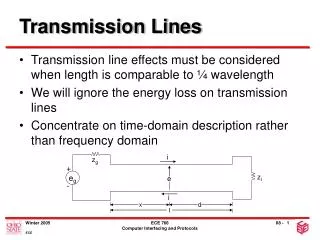
The Transmission Lines • Definition: • Structures used to transmit energy or signal in the form of guided-wave electromagnetic fields from one place to another • Modeling: • Distributed-element model • Electromagnetic model • Key Concepts: • Waves and properties
The Lumped-Element Model Zs IA A IB B Transmission Line Vs ZL • Lumped-element model for the entire transmission as seen from A-A´ and B-B´: A´ B´ L (KCL) (KVL) • Valid only if • L (length of the line) << (wavelength of the signal)
The Distributed-Element Model z z z z z z • Divide the entire transmission line into segments with length z<< • For each segment, postulate the lumped elements related to the series resistance, the parallel capacitance C, the series inductance, and the parallel conductance.
Derivation of the transmission line equations Consider one segment at position z along the line: Rz Lz I(z+z,t) I(z,t) V(z,t) Cz Gz V(z+z,t) z R: the combined resistance of the conductors per unit length in /m L: the combined inductance of the conductors per unit length in H/m G: the conductance of the insulation medium per unit length in 1/m C: the capacitance of the conductors per unit length in F/m Next Step: To establish relations among the currents and the voltages at z and z+ z
By application of KVL: Divided by z and let z 0: Eq. (1-1a) By application of KCL: Or divided by z and let z 0: Eq. (1-1b)
Comments on the transmission line equations (1-1a) (1-1b) • Eqs. (1-1), within the level of approximations, are partial differential equations (PDE) that governing the voltage and the current along the transmission lines. • The line parameters R, L, G, C are related to the physical properties of the transmission line and may be functions of position z. • Give the line parameters, solutions of the eqs. (1-1) describe the the voltage and the current along the transmission lines
Wave Equations Assume R,L,G,C are all constants Eq. (1-2a) Eq. (1-2b)
Wave Equations for Lossless Transmission Line If the line is lossless, then R=G=0, therefore Eq. (1-3a) Eq. (1-3b) Eq. (1-4) The velocity of the propagating wave Conclusion: The voltage and the current travel along the transmission line as governed by the wave equations (1-3)!
Solutions to the Wave Equation for Lossless Transmission Line Eq. (1-5a) Eq. (1-5b) Forward propagating wave Backward propagating wave Conclusion: The total voltage and the current are sum of the forward and the backward propagating waves along the transmission line as expressed in (1-5).
Example: Forward Propagating Wave t=0 z t=T z vT
Derivation of the Power Equation Multiply eq. (1-1a) by I(z,t), eq. (1-1b) by V(z,t), add: Eq. (1-6) Stored EM Energy Total Power Power Dissipation Net Power Flow=Power Dissipation+Change in Stored Energy!
Steady-State TL Equations Assume that the signal has reached sinusoidal steady-state, then Eq.(1-7a) Eq.(1-7b) Real functions of z and t Complex functions of z only being the frequency of the sinusoidal signal Furthermore: Eq.(1-8a) Eq.(1-8b)
Comments on the steady-state transmission line equations (1-8a) (1-8b) • Equations (1-8) are ordinary differential equations (ODE) governing the complex voltage and the current V(z) and I(z) along the transmission lines. • The complex V(z) and I(z) have no direct physical meaning. On the other hand, once the complex V and I are known, the physical time-dependent, real solutions can be obtained by using eqs. (1-7) Procedure for Sinusoidal Steady State Solutions Convert to Complex Domain Solve Complex Equations Convert to Real Domain
Complex Power Equation Question: What will be the equivalence of the power equation (1-2) in term of the complex voltage and current? Derivation: Multiply eq.(1-8a) by the complex conjugate of I and the complex conjugate of (1-8b) by V and add: Eq.(1-9) Physical interpretation of the complex power equation?
Consider the real voltage and current are linked to the complex current and voltage as The instantaneous power dissipation is The time-average of the power dissipation is Note that We have Eq.(1-10)
The time-average power dissipation is Eq.(1-10) Similarly, the time-average power flow is Eq.(1-11) The time-average stored electric and magnetic energies are Eq.(1-12) Eq.(1-13) Rewrite eq. (1-9) in terms of eqs. (1-10)-(1-13) Eq.(1-14)
Real Part of Eq. (1-14) Eq.(1-15) z Average power in=Average power out+Average power lost! Imaginary Part of Eq. (1-14) Eq.(1-16) If we define a complex power as then the real P(z) is the average power flow, and the imaginary P(z) is proportional to the difference in stored magnetic and electric energy densities. Eq.(1-17)
Steady-State Wave Equation (1-8a) (1-8b) If R,L,G,C are all constants of z, then by taking derivative of (1-8a) and making use of (1-8b), we have Eq. (1-18a) Similarly, we have Eq. (1-19) Complex Propagation Constant in 1/m Eq. (1-18b)
General Solutions Eq. (1-20a) Eq. (1-20b) Physical Meaning of the General Solution: The total voltage/current are sum of the forward (exp[-z]) and the backward (exp[-z]) propagating waves being constants to be determined
Relationship betweenV andI By substituting (1-20) into (1-8), we obtain Eq. (1-21) Zo: the characteristic impedance of the transmission line () Yo: the characteristic admittance of the transmission line (1/ ) Eq. (1-20a) Eq. (1-20b) Only two knowns V remain to be determined!
Semi-Infinite Line Zs Vs z 0 Suppose that the line extends to infinite along +z. Therefore, the backward propagating waves do not exist. We obtain Note that is complex and let =+j. We have
The instantaneous voltage and current are Eq. (1-22a) Eq. (1-22b) t=0 V(z,t) t=t1 z Amplitude: decay according to exp(-z), therefore is the amplitude decay constant of the wave Phase: advance according to (t-z), is a measure of the phase change per unit length along z, therefore the propagation constant
Phase Velocity Definition: The velocity at which the phase of the wave travels Let us observe a point of constant phase such that Take derivative with respect to time t Re-arrange so that that phase velocity is expressed as Eq. (1-23) Which is a function of frequency and dependent on the physical properties of the transmission line through .
Power Flow Instantaneous power flow: Eq. (1-24) Time-average power flow: Eq. (1-25) Note that the average power is dependent on the phase shift between the voltage and the current.