Download
1 / 13
130 likes | 223 Views
CERN Accelerator School Superconductivity for Accelerators Case study 6: RF test and properties of a superconducting cavity. GROUP B C. Darve S. Izquierdo Bermudez X. Niu K. Papke R. Santiago Kern. Elliptical 5-cell cavity in pi-mode: Basic Parameters (I). 1. Energy of the protons:.

E N D
CERN Accelerator SchoolSuperconductivity for AcceleratorsCase study 6:RF test and properties of a superconducting cavity GROUP B C. Darve S. Izquierdo Bermudez X. Niu K. Papke R. Santiago Kern
Elliptical 5-cell cavity in pi-mode: Basic Parameters (I) 1. Energy of the protons: 2. Distance between two neighbouring cells (L) and length of the cavity (Lacc) Case study 6
Elliptical 5-cell cavity in pi-mode: Basic Parameters (II) 3. All the given parameters depend ONLY in the geometry of the cavity Remark 1: Typically, for elliptical cells β=[0.6,0.8] and Epk/Eacc=[2,2.6] Cavities with elliptical cells for low beta become very big as lower frequencies are used and less stable mechanically (the accelerating gap shortens and cavity walls become more vertical) Remark 2: In circular accelerators the factor Ra/Q is usually defined as: Case study introduction
RBCS 4. The cavity is made of SC Nb operating at 2 K. RBCS can be approximated to f=704.4 MHz Tc(Nb)=9.2 K T • Operating the cavity at 2 K means lower RCBS, which in turn gives a higher Qo • If we look at the experimental correlation: • a. ->BCS • b. ->BCS • But the reality is much more complex! Case study introduction
Quality Factor Qo • For a real cavity, the residual resistance should be taken into account. • The possible contributions to Rres: • Trapped magnetic field • Normal conducting precipitates • Grain boundaries • Interface losses • Subgap states • RRR? Typically (0.5 achievable?) Case study introduction
Accelerating and maximum gradient (I) 7. Maximum gradient that can be achieved in this cavity If we take 190 mT as the critical magnetic RF surface field at 2 K = 34 MV/m Magnetic field Expected location of the Magnetic quench z Case study introduction 6. Operation @ stored energy of 65 J i) Accelerating gradient ii) Dissipated power in the cavity walls
Accelerating and maximum gradient (II) Eacc (14.2 MV/m) < Emax (34 MV/m) • We are operating at half of the maximum accelerating gradient. Is this standard? • Of course, we don’t wont to work at Emax any perturbation in the system will involve a quench: Cooling power is able to compensate: nothing happens Pdis Heat source ∆T Magnetic quench • Possible sources: • Surface defects • Bad cooling • Multipacting • Field emission Case study introduction
Loaded Quality Factor QL QL We will be able to tune the cavity within this range Δω Case study introduction Loaded quality factor: + W=65 J ; Pext=100 kW W is the energy stored in the cavity Qextdescribes the effect of the power coupler attached to the cavity Pext is the power exchanged with the coupler. QL of the cavity. + = 2.88x10⁶ Frequency bandwidth of the cavity.
Tuners FREQUENCY TUNERS: Keep the frequency of the cavity on its nominal value. • Stepper motor tuners: for coarse tuning, they are slow in response (i.e. when the cavity is cooled down) • Piezo-tuners: for fine tuning, fast response (i.e. to accommodate for vibrations and pressure fluctuations from the He bath). The control of the piezo tuners is done by comparing the phase difference between reflected and forward signals H. Saugnac SLHiPP2 Case study introduction
Impact of a normal conducting incursion • Local Surface resistant at the defects much higher • Mean surface resistance Rs (averaged over the surface) increased • The impact will be different depending in the location! Critical magnetic RF surface field defect (piece of copper) Especially in high magnetic field regions, defects lead to high energy dissipation Defects of 1µm already have an impact! R over Q Case study 6
Additional questions (I) Let’s assume that we are thinking about a high field accelerator quality magnet • High temperature superconductor: YBCO vs. Bi2212 • Bi2212: • We can produce round wires with multifilamentary configuration • Mechanically instability is still an issue • YBCO: • Seems very promising, lower cost? • But… • Strongly anisotropic • Nowadays only available in tapes and lot of open questions • Effect of transverse stress? • AC losses/ transient effects on field quality No significant differences in terms of critical surface/penetration depth in between Bi2212/YBCO Our choice: Bi2212 Case study 6
Additional questions (II) • Superconducting coil design: block vs. cos • cos • Use the beam pipe as inner support • More flexibility: dipole, quadrupole, sextupole… • Ratio central field/current density is more with the same quantity of cable. • Block • Easier to wind • For the case of a dipole, simple way to achieve good field quality...but mechanical support can be an issue Our choice: cos • Support structures: collar-based vs. shell-based If the field is very high, you need higher pre-stress after cool down…so the bladders/shell-based solution should be better. Still lot of development needed to assure mechanical stability at 20T! Our choice: shell-based
Additional questions (III) • Assembly procedure: high pre-stress vs. low pre-stress • We always want to apply sufficient pre-stress to assure that all the cables are under compression in operation conditions. • During the R&D phase, one should look at maximum pre-stress can be applied before degradation and stays bellow this value. • For production, to assure reproducibility, one should keep some margin (about 20%-40%) from this upper boundary. If the pre-stress is very low, reproducibility might become an issue?