Download
1 / 54
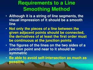
540 likes | 659 Views
Solution Space Smoothing Method and its Application. Dong Sheqin Hong Xianlong 董社勤 洪先龙 Department of Computer Science and Technology, Tsinghua University, Beijing,100084 P.R. China. Outline. Principle of Search Space Smoothing VLSI Placement based on SSS

E N D
Solution Space Smoothing Method and its Application Dong Sheqin Hong Xianlong 董社勤 洪先龙 Department of Computer Science and Technology, Tsinghua University, Beijing,100084 P.R. China
Outline • Principle of Search Space Smoothing • VLSI Placement based on SSS • Local Smoothing & Global Smoothing • VLSI Placement based on P-SSS • Experimental Results • Applications: TSP, Temporal planning, FPGA Floorplanning
NP-hard Problem and Optimization Algorithm • A NP-Hard Problem has a complicated search space, a greedy search strategy gets stuck at one of the deep canyons easily, unable to climb out and to reach the global energy minimum. • To avoid getting stuck at one local minimum, there are commonly two types of approaches. 1). To introduce complex moves, 2). To introduce some mechanisms to allow the search to climb over the energy barrier. (ie. The simulated annealing algorithm)
History of Search Space Smoothing (SSS) • Jun Gu and Xiaofei Huang proposed a 3rd approach, that is, to smooth the solution space. • They had applied this method to the classical NP-hard problem: TSP. Using the smoothing function below.
Principle of Search Space Smoothing • By Search Space Smoothing ,The rugged terrain of search space of a NP-hard problem is smoothed, and therefore the original problem instance is transformed into a series of gradually simplified problem instances. The solutions of the simplified instances are used to guide the search of more complicated ones. Finally, the original problem is solved in the end of the series.
Formal Description of SSS Algorithm //Initialization α ← α0; x ← x0; //Search while (α >= 0) do begin H(α)← DoSmooth(α, H); for (some times) do begin x’ ← NeighborhoodTransition(x); if (Acceptable(α, x, x’)) then begin x ← x’; end; end; α ← NewAlpha(α); end; End;
History of Search Space Smoothing (SSS) • Johannes Schneider investigates this method for traveling salesman problem thoroughly and pointed out that “the advantage(of search space smoothing) over the later one(simulated annealing: SA) is that a certain amount of computational effort usually provides a better result than in the case of SA” • SSS + SA is infeasible proved by analytic and experimental results of Johannes Schneider
Summary of The Principle of SSS • To solve the original Problem instance Pi, SSS first transform Pi to a series of Problem instance Pi0, Pi1 , Pi2 , Pi3 , Pi4 …….. • it is obvious that Pi0 is similar to Pi1 , Pi1 is similar to Pi2 , and so on. In some sense, the “distance” between Pi0 and Pi1 is smaller than the “distance” between Pi0 and Pi2. • Obviously, the optimal solution of Pi1 is very close to the optimal solution of Pi0 in some sense. Because the two problem instances have great similarity. • In the series, each problem instance is a gradually smoothed approximation of the previous problem instance in some sense.
Outline • Principle of Search Space Smoothing • VLSI Placement based on SSS • Local Smoothing & Global Smoothing • VLSI Placement based on P-SSS • Experimental Results • Applications: TSP, Temporal planning, FPGA Floorplanning
CPU PLA I/O ROM/ RAM A/D Problem of VLSI Placement • A Soc is composed of IPs and Macro building blocks • The first step to physically design a Soc is constraint driven floorplanning and placement.
How to smooth the search space for a Placement instance--an example • Incremental optimization
How to smooth the search space for a Placement instance--an example • Placement instance smoothing(their optimal solution must be very close to each other)
The basic smoothing function • To calculate the first placement instance by left formula • To calculate the successive placement instances by the formula below:
Outline • Principle of Search Space Smoothing • VLSI Placement based on SSS • Local Smoothing & Global Smoothing • VLSI Placement based on P-SSS • Experimental Results • Applications: TSP, Temporal planning, FPGA Floorplanning
Global Smoothing • For a placement instance which has 4 modules, their sizes are 2 * 1.8, 2 * 1.8,1.8 * 0.5, 1.8 * 0.5, and the corresponding numbers are 1, 2, 3, 4. The global optimal solution is depicted as Fig.1(a), we name it as solution-1. Obviously, another solution depicted as Fig.1(b) is not a global optimal solution, we name it as solution-2. For a BSG as Fig.1(c), if we place modules 2 * 1.8, 2 * 1.8, 1.8 * 0.5, 1.8 * 0.5, their corresponding numbers are 1, 2, 3, 4, in Fig.1(c) BSG in (2,2), (3, 2), (2, 1), (3, 1), we get a local minimum (solution-2). If we use greedy search described above, there is no way to achieve the global optimal solution from this local minimum. • However, if we “smoothed” the placement instance that the four modules have the same size, solution-1 and solution-2 will both be the global optimal solutions of the “smoothed” placement instances. Note that, original placement instance (2 * 1.8, 2 * 1.8, 1.8 * 0.5, 1.8 * 0.5), smoothed to placement instance (2 * 1.8, 2 * 1.8, 2 * 1.8, 2 * 1.8), or (1.8 * 0.5, 1.8 * 0.5, 1.8 * 0.5, 1.8 * 0.5), the later two “smoothed” instances are similar to the original instance, their solution spaces are also similar to the solution space of the original placement instance, but the number of local minimums are reduced in the “smoothed” solution spaces.
Global Smoothing • Definition 1: Suppose the neighborhood of a solutionis, is a local minimum, iff • After smoothed with parameter α, we say the local minimumis eliminated, iff
Local effect of the smoothing operation • We first randomly choose tens of different solutions, and for each solution si, randomly select 1000 other solutions sj (j = 1, 2, …, 1000) within its neighborhood N(si). For every α, we calculate the energy (area, for Placement Problem) differences: • Then the Root-Mean-Square (RMS) value of all the 1000 energy differences is:
Local Smoothing • Definition 2: Suppose the neighborhood of a solution s0 is, and the size of the neighborhood is : • And we have a vector of energy differences • Then the local smoothness of could be described by:
How to make use of Global Smoothing effect in SSS • For Greedy Local Search, Suppose there are two solutions si and sj within a neighborhood, , then the probability of accepting the transition is • For the global smoothing effect, which changes the sign of energy difference of some pairs of solutions, the greedy strategy is effective, but as to the local smoothing, greedy strategy is completely insensitive to it.
How to make use of Local smoothing effect • In Simulated Annealing, Metropolis algorithm is used to make a quasi-equilibrium state at a given temperature t. • Obviously, , for . could be viewed as the smoothed result of energy difference under control parameter t. , .
How to make use of Local smoothing effect • A local search, which is sensitive to both global and local smoothing effects, would leads to a better result. • The Metropolis function that have a smooth transition from 1 to 0 of the accepting probability should be introduced and the local search algorithm could degenerate to greedy algorithm in the original un-smoothed search space for convergence reason.
A Local search that can make use of local smoothing • A Local search with a proper accepting probability can make use of both global smoothing effect and local smoothing effect
Outline • Principle of Search Space Smoothing • VLSI Placement based on SSS • Local Smoothing & Global Smoothing • VLSI Placement based on Probability Search Space Smoothing • Experimental Results • Applications: TSP, Temporal planning, FPGA Floorplanning
Algorithm: Probability-SSS () • STEP 1: create the initial placement instance according to the smoothing function. • STEP 2: use a local search with probability acceptance function to search the solution for the initial placement instance. The result is a starting solution. • STEP 3: α ← NewAlpha(α) ; apply the smoothing function to the previous solution to produce a new placement instance. • STEP 4: use local search algorithm a local search with probability acceptance function to search the solution for the new placement instance. The result is the current solution. • STEP 5: if =0, stop. The current solution is the final solution. Otherwise, using the current solution, go to STEP 3.
Outline • Principle of Search Space Smoothing • VLSI Placement based on SSS • Local Smoothing & Global Smoothing • VLSI Placement based on Probability Search Space Smoothing • Experimental Results • Applications: TSP, Temporal planning, FPGA Floorplanning
Experimental Results: placement example ami33(1)- area usage is 98.85%
Experimental Results: placement example ami49 - area usage is 98.85%
Outline • Principle of Search Space Smoothing • VLSI Placement based on SSS • Local Smoothing & Global Smoothing • VLSI Placement based on Probability Search Space Smoothing • Experimental Results • Applications: TSP, Temporal planning, FPGA Floorplanning
Application:Using P-SSS to solve TSP • Solution quality (excess over optimal solution )
3D-BSSG representation Application: FPGA Temporal Planning using P-SSS
Experimental Results • Cost Function: Φ = Volume + β * Wirelength • Temporal precedence requirements, which describe the temporal ordering among modules, should also be satisfied in our algorithm. • Using 3D-MCNC benchmarks, two groups of experiments are performed.
Experimental Results • In the first experiment, our objective is to compare P-SSS with G-SSS as the quantity of precedence constraints varies. • Conclusions from this experiment. • The increase of the precedence constraints number leads to decrease of the quality of search. • Combination with Metropolis algorithm makes SSS more powerful than that with Greedy algorithm as local search method.
Experimental Results • Experimental results on all circuits of 3D-MCNC • Conclusion: P-SSS algorithm improve over G-SSS algorithm in both volume and wirelength
Experimental Results • In the second experiment, using same benchmarks and same constraints, we respectively execute the Simulated Annealing approach and P-SSS algorithm based on two kind of representation: 3D-subTCG and Sequence Triplet (ST).
Application:Heterogeneous FPGA Floorplanning Based on Instance Augmentation
Instance Augmentation • Instance Augmentation is a new stochastic optimization method, which showed great ability in constrained floorplanning, such as fixed-outline floorplanning [Rong Liu, ISCAS05]. • Floorplanning for heterogeneous can be regarded as a constrained floorplanning problem: • fixed-outline, since size of the device is fixed; • Each module’s requirement for all kinds of resources must be satisfied. • Therefore, we applied IA on heterogeneous floorplanning problem.
Overview • Start from sub-instance of the given instance. That is, it first floorplans a subset of the given modules. • Simulated annealing or greedy local search may be adopted to find feasible solutions of specific instance. • When feasible solution of sub-instance is found, augment it by inserting modules (called down-casting). • If no feasible solution of current sub-instance is found, “shrink” it by removing a module (called up-casting). Illustration of so called instance augmentation
Overview Note: a solution is feasible iff all the modules of the instance are put into the device and their requirement for all kinds of resources fulfilled. Main flow of Instance Augmentation
Some Details • Once augment a sub-instance to a bigger one, an initial solution of the bigger instance is also generated by inserting the module to the feasible solution of the sub-instance. For example: (abcd, badc) -> (aebcd, baedc) • Different inserting positions and realizations of the module is tried to find a better insertion. Experiments show that lots of feasible solutions can be obtained directly by this way.
Some Details • When “shrink” current instance to a smaller one, an initial solution of the smaller instance is also generated by removing the module to the feasible solution of the sub-instance. For example: (aebcd, baedc)->(abcd, badc) • To avoid the algorithm stuck in local minimum, there may be more than one module be removed when “shrink” current instance.
Some Details • Either simulated annealing or greedy local search can be used to search for feasible solution of current instance; • This work adopted simulated annealing; • Since the initial solutions often have good qualities, simulated annealing used here has: • very low start temperature; • few iterations at each temperature;
Some Details • Inserting small modules has less destruction to the floorplan than inserting large modules. • Therefore, we • sort the modules by their requirements for resources in descending order; • insert modules in this order; • Experiments prove that inserting modules in this order induce higher success-ratios.
Problem Definition • Heterogeneous FPGA device • Instead of being composed of similar CLBs, modern FPGA devices have more heteroge-neous logical resources. • Xilinx’s Vertix II and Spartan 3 families are typical heterogeneous FPGA devices. Simplified architecture of Xilinx’s XC3S5000, which is composed of CLBs, RAMs and Multipliers.