Download
1 / 64
640 likes | 652 Views
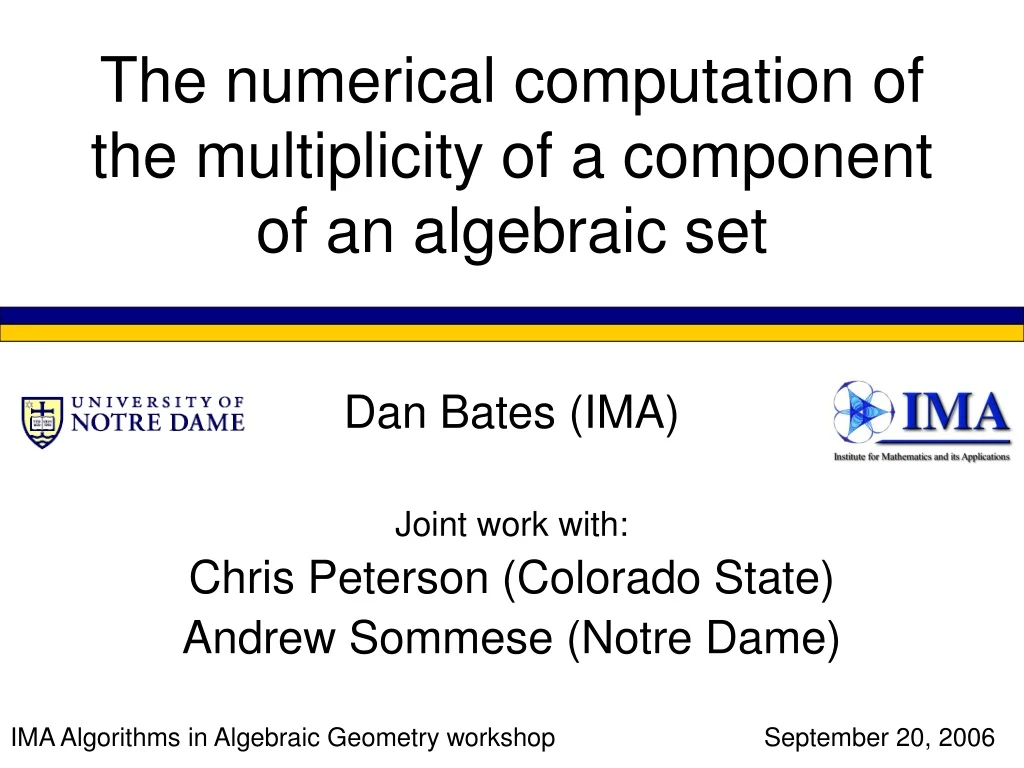
The numerical computation of the multiplicity of a component of an algebraic set. Dan Bates (IMA) Joint work with: Chris Peterson (Colorado State) Andrew Sommese (Notre Dame) IMA Algorithms in Algebraic Geometry workshop September 20, 2006. Contents. Motivation Background The method

E N D
The numerical computation of the multiplicity of a component of an algebraic set Dan Bates (IMA) Joint work with: Chris Peterson (Colorado State) Andrew Sommese (Notre Dame) IMA Algorithms in Algebraic Geometry workshopSeptember 20, 2006
Contents Motivation Background The method Complete examples A few implementation details Other examples A similar method 1/27
Motivation Basic problem: Compute the regularity and multiplicity of a 0-scheme supported at a single point. 2/27
Motivation Basic problem: Compute the regularity and multiplicity of a 0-scheme supported at a single point. Why we got involved: To develop algorithms for computing numerical free resolutions, we needed to know which degrees could appear among the syzygies. 2/27
Motivation Basic problem: Compute the regularity and multiplicity of a 0-scheme supported at a single point. Why we got involved: To develop algorithms for computing numerical free resolutions, we needed to know which degrees could appear among the syzygies. In other words, we needed a way to compute regularity. Multiplicity came for free! 2/27
Motivation Why would anyone else care about regularity or multiplicity? 3/27
Motivation Why would anyone else care about regularity or multiplicity? Here are 3 answers: 1. Like I said, regularity bounds the degrees that syzygies could have, so regularity is a stopping criterion. 3/27
Motivation Why would anyone else care about regularity or multiplicity? Here are 3 answers: 1. Like I said, regularity bounds the degrees that syzygies could have, so regularity is a stopping criterion. 2. Multiplicity is intrinsic to the polynomial system. In some settings, it is the number of paths leading to the point during homotopy continuation. 3/27
Motivation 3. Numerical primary decomposition. The witness sets of numerical algebraic geometry provide a kind of numerical primary decomposition of the radical. These witness points are found by slicing the algebraic set with hyperplane sections. 4/27
Motivation 3. Numerical primary decomposition. The witness sets of numerical algebraic geometry provide a kind of numerical primary decomposition of the radical. These witness points are found by slicing the algebraic set with hyperplane sections. One step towards the numerical primary decomposition of the original ideal is to retain the scheme structure when slicing. 4/27
Motivation Q: Why not just use symbolic methods? 5/27
Motivation • Q: Why not just use symbolic methods? • A: Here are two reasons: • Coefficient blowup (and other computational difficulties). 5/27
Motivation • Q: Why not just use symbolic methods? • A: Here are two reasons: • Coefficient blowup (and other computational difficulties). • Inexact input (since the polynomial system may contain random complex numbers and the point is almost surely inexact). 5/27
Motivation The point of this talk: - Can compute the multiplicity and the regularity of a 0-scheme supported at a single point numerically 6/27
Motivation The point of this talk: - Can compute the multiplicity and the regularity of a 0-scheme supported at a single point numerically - No coefficient blowup 6/27
Motivation The point of this talk: - Can compute the multiplicity and the regularity of a 0-scheme supported at a single point numerically - No coefficient blowup - Works under small perturbations 6/27
Motivation There are actually two related methods: ● B., Peterson, and Sommese (see [BPS]): Inspired by known modern symbolic methods; uses a regularity criterion of Bayer and Stillman (see [BS]) to know when to stop ● Dayton and Zeng (see [DZ]): Inspired by the duality approach of Macaulay; relies on the use of structured matrices The two methods each give the multiplicity, but the other output differs…. 7/27
Background What is multiplicity? Multiplicity you have seen, e.g., x2. It is the number of times a component should be counted. 8/27
Background What is multiplicity? Multiplicity you have seen, e.g., x2. It is the number of times a component should be counted. It can be extracted from the Hilbert polynomial. 8/27
Background What is regularity? This is more subtle. 9/27
Background What is regularity? This is more subtle. The regularity tells us a point at which the Hilbert function stabilizes. 9/27
Background Basic setup: ● I = {f1, f2, …, fr} is a homogeneous ideal. 10/27
Background Basic setup: ● I = {f1, f2, …, fr} is a homogeneous ideal. ● I is supported at a single point p in Pn. 10/27
Background ( ) Basic setup: ● I = {f1, f2, …, fr} is a homogeneous ideal. ● I is supported at a single point p in Pn. Note: I could be produced by slicing a positive-dimensional irreducible component with generic hyperplanes: multiplicity is preserved, regularity is not. 10/27
Background ( ) Basic setup: ● I = {f1, f2, …, fr} is a homogeneous ideal. ● I is supported at a single point p in Pn. Note: I could be produced by slicing a positive-dimensional irreducible component with generic hyperplanes: multiplicity is preserved, regularity is not. ● R = C[x0, x1, …, xn]. 10/27
Background ● (I)kis the degree k homogeneous part of I. 11/27
Background ● (I)kis the degree k homogeneous part of I. ● Ip is the prime ideal at the point p. 11/27
Background ● (I)kis the degree k homogeneous part of I. ● Ip is the prime ideal at the point p. ● (I:F) = {G in R | GF is in I} is the ideal quotient of I by F (where F is in R). 11/27
Background ● (I)kis the degree k homogeneous part of I. ● Ip is the prime ideal at the point p. ● (I:F) = {G in R | GF is in I} is the ideal quotient of I by F (where F is in R). ● The saturation of I is the intersection of all primary ideals in a reduced primary decomposition of I that are not m-primary (i.e., those that have geometric content). 11/27
Background Key theorem (Bayer and Stillman, 1987): 12/27
Background Key theorem (Bayer and Stillman, 1987): Suppose I is generated in degree at most m. 12/27
Background Key theorem (Bayer and Stillman, 1987): Suppose I is generated in degree at most m. Then the following are equivalent: reg(I) = m. 12/27
Background Key theorem (Bayer and Stillman, 1987): Suppose I is generated in degree at most m. Then the following are equivalent: reg(I) = m. (something) 12/27
Background Key theorem (Bayer and Stillman, 1987): Suppose I is generated in degree at most m. Then the following are equivalent: reg(I) = m. (something) (something else) 12/27
Background Suppose I (homogeneous) is generated in degree at most k, vanishing only at the point p in Pn. Let L be a linear form not contained in Ip. Then reg(I) ≤ k if and only if (I:L)k=(I)k and (I, L)k=(R)k. Corollary (to Bayer and Stillman, 1987): 13/27
The Algorithm (roughly) A 0-scheme consists of a point and some multiplicity structure around the point. Our idea is to look at successively larger infinitessimal neighborhoods around the point until all multiplicity information is captured. This is similar to computing the multiplicity of a monomial ideal using the “staircase” method. 14/27
Background Two other facts: 1. Suppose Ip is an associated, non-embedded prime of an ideal I (p a point in Pn). Let Jk = (I, Ipk). Then the multiplicity of I at Ip is equal to the multiplicity of Jk at Ip for k >> 0. 2. If the multiplicity of Jk at Ip is equal to the multiplicity of Jk+1 at Ip, then the multiplicity of I at Ip is also equal to the same. 15/27
Background As mentioned before, if regularity is known, then computing the multiplicity is trivial: μ = dim(R/I)k for k >> 0. Which k suffices? k = reg(I). 16/27
The Algorithm (detailed) INPUT: I={F1, …, Fr} homogeneous in R (n+1 variables) and the point p at which I is supported (with the final coordinate of p being nonzero, WLOG). OUTPUT: Multiplicity and regularity. Let Ip = {pizj - pjzi | 0 ≤ i,j ≤ n}. Let m = (z0, …, zn). Let k = maximal degree in which I is generated, μ(k-1) = -2, and μ(k) = -1. 17/27
While μ(k) ≠ μ(k-1)do: - Form Ipk, Jk=(I, Ipk), znmk. Let A=0, B=1. - While A ≠ B do: - Form (Jk)k+1. - Compute P = (Jk)k+1∩ znmk. - Compute the preimage P’ of P. - Compute A = rank((Jk)k), B = rank(P’). - If A = B, μ(k) = rank((m)k) – A; else let Jk = P’. - If μ(k) = μ(k-1), then μ = μ(k) and reg(I) ≤ k; else increment k. 18/27
Complete examples Example: I = (x2, y) in the variables (x, y, z) at the point (0, 0, 1). Ip = (x, y). m = (x, y, z). k = 2, μ(2) = -2, and μ(3) = -1 19/27
Complete examples Example: I = (x2, y) in the variables (x, y, z) at the point (0, 0, 1). Ip = (x, y). m = (x, y, z). k = 2, μ(2) = -2, and μ(3) = -1 After some work at the board: μ = 2 and reg(I) = 3. 19/27
Complete-ish examples Example: I = (x2, y3) in the variables (x, y, z) at the point (0, 0, 1). 20/27
Complete-ish examples Example: I = (x2, y3) in the variables (x, y, z) at the point (0, 0, 1). k = 3: A=5, B=5, so μ(3) = 10-5 = 5. 20/27
Complete-ish examples Example: I = (x2, y3) in the variables (x, y, z) at the point (0, 0, 1). k = 3: A=5, B=5, so μ(3) = 10-5 = 5. k = 4: A=9, B=9, so μ(4) = 15-9 = 6. 20/27
Complete-ish examples Example: I = (x2, y3) in the variables (x, y, z) at the point (0, 0, 1). k = 3: A=5, B=5, so μ(3) = 10-5 = 5. k = 4: A=9, B=9, so μ(4) = 15-9 = 6. k = 5: A=15, B=15, so μ(5) = 21-15 = 6. 20/27
Complete-ish examples Example: I = (x2, y3) in the variables (x, y, z) at the point (0, 0, 1). k = 3: A=5, B=5, so μ(3) = 10-5 = 5. k = 4: A=9, B=9, so μ(4) = 15-9 = 6. k = 5: A=15, B=15, so μ(5) = 21-15 = 6. So μ = 6 and reg(I) = 4. 20/27
Implementation Details After fixing a term order, homogeneous polynomials may easily be represented as vectors of coefficients. 21/27
Implementation Details After fixing a term order, homogeneous polynomials may easily be represented as vectors of coefficients. Most steps of the algorithm are very straightforward symbolic maneuvers. 21/27
While μ(k) ≠ μ(k-1)do: - Form Ipk, Jk=(I, Ipk), znmk. Let A=0, B=1. - While A ≠ B do: - Form (Jk)k+1. - Compute P = (Jk)k+1∩ znmk. - Compute the preimage P’ of P. - Compute A = rank((Jk)k), B = rank(P’). - If A = B, μ(k) = rank((m)k) – A; else let Jk = P’. - If μ(k) = μ(k-1), then μ = μ(k) and reg(I) ≤ k; else increment k.