Download
1 / 9
90 likes | 104 Views
The ONR Physical Oceanography Code 32 DRI Workshop aims to understand lateral mixing and coherent turbulence at various scales through field work, modeling, and technology innovation.

E N D
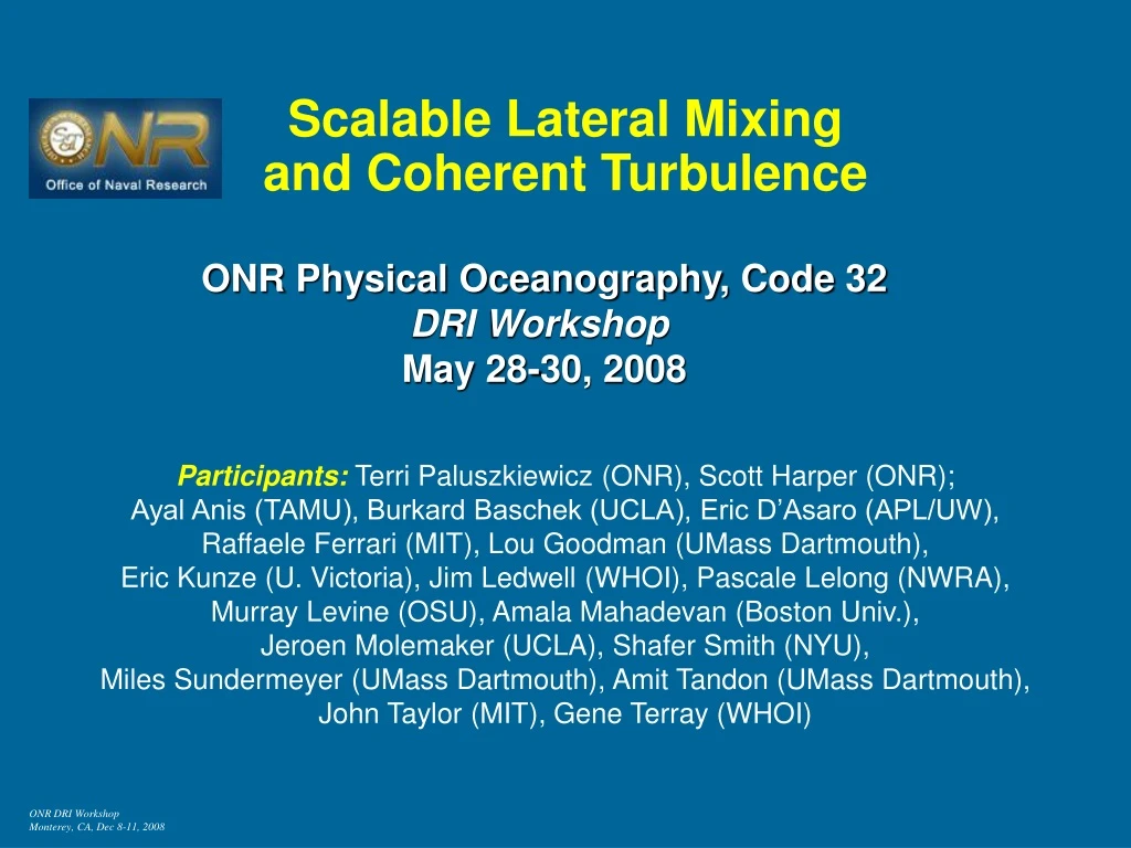
Scalable Lateral Mixing and Coherent Turbulence ONR Physical Oceanography, Code 32 DRI Workshop May 28-30, 2008 Participants:Terri Paluszkiewicz (ONR), Scott Harper (ONR); Ayal Anis (TAMU), Burkard Baschek (UCLA), Eric D’Asaro (APL/UW), Raffaele Ferrari (MIT), Lou Goodman (UMass Dartmouth), Eric Kunze (U. Victoria), Jim Ledwell (WHOI), Pascale Lelong (NWRA), Murray Levine (OSU), Amala Mahadevan (Boston Univ.), Jeroen Molemaker (UCLA), Shafer Smith (NYU), Miles Sundermeyer (UMass Dartmouth), Amit Tandon (UMass Dartmouth), John Taylor (MIT), Gene Terray (WHOI)
May 2008 DRI Workshop Goals • Formulate DRI - emphasis on 3 year field program, 2 years analysis • Generate straw-plan for field work • Modeling, theory, and technology innovation: What must happen? • What pathways must be pursued to achieve objectives and enable field work
Proposed DRI Priorities / Hypotheses • Main Goal: To better understand lateral mixing at scales of 10 m – 10 km • Primary Hypotheses: • 1. Inhomogeneous IW mixing creates PV anomalies that are responsible for • significant isopycnal mixing. • 2. Mesoscale straining leads to a cascade of both tracer and PV variance to • submesoscales that is responsible for significant submesoscale isopycnal • mixing. • 3. Non-QG, submesoscale instabilities feed a forward cascade of energy, • scalar and PV variance which enhances both isopycnal and diapycnal mixing.
Proposed DRI Priorities / Hypotheses (cont’d) Secondary Hypotheses: 4. Submesoscale variability is associated with coherent structures: mixing is inhomogeneous and anisotropic and submesoscale processes are inherently vertical as well as horizontal. 5. "Fronts are not barriers to transport". Specifically, we hypothesize that submesoscale processes facilitate cross-density-front exchange (Here, the point is to understand how a collection of submesoscale processes add up to give a cross-front transport at the mesoscale; i.e. bolus transport, not mixing that leads to irreversible mixing - diffusion). 6. Filaments develop a slope of f/N at scales dominated by geostrophic dynamics. (What sets the width and thickness of filaments?) 7. The lateral downscale variance cascade is absorbed by vertical (as opposed to lateral) mixing processes. How does filamentation interact with vertical processes, e.g., double diffusion, Kelvin-Helmholtz, internal wave breaking?
Field Site Selection • Strategy • Identify key features of mechanisms of interest • Identify regions of ocean that provide strongest signal and highest probability of exhibiting those phenomena • Recommended two sites • To obtain contrast between regions of low and high eddy energy • To provide end-points for mechanisms of interest, from which modeling studies can determine role of each process under varying intermediate conditions • Site 1 should be in midst of mesoscale eddy field of moderate eddy kinetic energy, away from influence of coast and persistent fronts • Site 2 should be at location with high likelihood of strong frontal activity, and associated high available potential energy • For both sites, a number of factors should be taken into account when choosing a specific geographic region and time of year (see white paper)
B A Open Ocean Site: Field Site 1 • Patch of water ~200 km across, accessible by ship and aircraft, most likely from an island • Field campaign of 3-4 weeks duration, in 2nd year of DRI • Characterize using satellite observations, and possibly aerial and ship surveys and/or AUVs • Smaller study sites within, on the order of 10 km across
Frontal Site: Field Site 2 • Very strong gradients and submesoscale instabilities compared to the generic open ocean conditions of field site 1 • Field campaign of 3-4 weeks duration, in 3nd year of DRI • Observational program consisting of: • Lagrangian mapping, • Eulerian mapping, • Float/glider mapping, • Microstructure measurements, • Remote sensing
Numerical Modeling and Theory • Multi-scale modeling to cover range of dynamical regimes and scales • QG models • primitive equation hydrostatic and non-hydrostatic models • Boussinesq models • large eddy simulation • Hierarchical process studies and/or grid nesting to span scales and dynamical regimes • Regional and process study modeling preceding the field experiments • Following field experiments, realistic and process-study models to: • interpret the observations • extend hypotheses over wider parameter range • examine specific and statistical conditions at study sites • distinguish different processes of interest • Operational regional models to: • forecast and hindcast actual conditions in field • provide boundary conditions (deterministically and statistically) for process study models
Proposed DRI Timeline • FY09 • Set up models • Continue instrument development • Initial field testing • FY10 • Field studies (Site 1) • Process modeling • Additional instrument development • Additional testing for year 3 • FY11 • Field studies (Site 2) • Process modeling • FY12 • Post experiment analysis • Process modeling • FY13 • Analysis / synthesis • Report findings