Download
1 / 32
410 likes | 1.01k Views
Turbulence and mixing in estuaries. Rocky Geyer, WHOI Acknowlegments : David Ralston, WHOI Malcolm Scully, Old Dominion U. wind. Wind-driven turbulence. velocity. Interfacial, shear-driven turbulence. Boundary-layer turbulence. Simplest case: unstratified tidal flow:

E N D
Turbulence and mixing in estuaries Rocky Geyer, WHOI Acknowlegments: David Ralston, WHOI Malcolm Scully, Old Dominion U.
wind Wind-driven turbulence velocity Interfacial, shear-driven turbulence Boundary-layer turbulence
Simplest case: unstratified tidal flow: Only boundary-layer turbulence Velocity = log layer “eddy viscosity” stress ub Bottom stress τB /ρ=Cdub2=u*2 Turbulent velocity scale uT~u* ~ 0.05 ub
Mixing Length model for the Eddy Viscosity / Diffusivity from log layer observations: define:
“reduced” gravity Now add stratification Buoyancy frequency Velocity “eddy viscosity” ρ1 enhanced shear near pycnocline stratification damps turbulence near pycnocline ρ2 stress ub log layer near bottom
What is the maximum vertical scale for turbulence with stratification? Bernoulli Function (energy-conserving flow) z The Ozmidov scale: maximum size of eddies before gravity arrests them.
Schematic of turbulence length-scale in a stratified estuary turbulence suppressed Ozmidovscaling: LT=uT/N distance from bed u(z) Boundary layer: LT ~ kz
Limiting Length-scales in Turbulent Flows Boundary-Layer Scaling (depth limiting) Ozmidov Scaling (stratification limiting) h LT z Note that LT Thorpe overturn scale 0 0.2 h LBL
Relative flow direction
ko spectral density S(k) Turbulence length-scale LT~ 1/ko
Scully et al. (2010) Influence of stratification on estuarine turbulence Snohomish River Boundary-Layer scaling Ozmidov Length scaling
ko Dissipation: the currency ($ or € ?) of turbulence ensemble average of turbulent motions Turbulent dissipation (conversion of turbulent motions to heat) = In a boundary layer, dissipation ~ production “Inertial subrange” method for estimating dissipation:
The Parameter Space of Estuarine Turbulence Estuaries Rivers 3 m 30 cm lo =1 m 3 cm 10 cm Turbulent Dissipation ε, m2s-3 Continental Shelf Lakes Viscous limit Ocean lo = ( ε/N3 )1/2 Geyer et al. 2008: Quantifying vertical mixing in estuaries Buoyancy Frequency N, s-1
Two different paradigms of estuarine mixing. How important is the stratified shear layer paradigm in estuarine turbulence? Stratified boundary layer Stratified shear layer turbulence turbulence u(z) u(z) no turbulence turbulence
Shear Instability Thorpe, 1973 gradient Richardson number Richardson, 1920 Smyth et al., 2001 necessary condition for stability Miles, 1961; Howard, 1961
Momentum balance of a tilted interface us ρ1 hi ρ2 ub 0.5-1x10⁻⁴ m2s-2 for strong transition zones – moderate but not intense stress
Fraser River salt wedge—early ebb (Geyer and Farmer 1989) interface 1.2 m/s meters weak motion bottom
Connecticut River: Geyer et al. 2010: Shear Instability at high Reynolds number 1.2 m/s Ri<0.25 leadingto shear instability 200 180 m 160 400 200 m 0
Day 325--Transect 17 (~ hour 19.1) river ocean Salinity meters along river dissipation of TKE dissipation of salinity variance
M M M Echo Sounding at Anchor Station B B B C C C M M B: braid C: core M: mixing zone M M M M #4 Salinity contours (black) Salinity variance (dots) #5 B B C C C B M #6 M M #4 Salinity timeseries ~ 60 seconds #5 M M M B B #6 B M M M C C C
Re~1,000 MIXING in cores Re~500,000 MIXING in braids
α ρ1 ρc ρ2 Baroclinicity of the braid accelerates the shear… with plenty of time within the braid… …leading to mixing:
New profiler data and acoustic imagery 20 seconds 30 meters
Very intense, and very pretty… 100 m …but is mixing at hydraulic transitions important at the scale of the estuary?
Buoyancy flux B = ∫∫∫β g s′w′ dV fresh Net Tidal Power “P” salt Dissipation D = ∫∫∫ε dV Energy balance: P = B + D Efficiency Rf = B/P = B/(D+B)
Hudson: ROMS Merrimack: FVCOM Massachusetts
Merrimack River mixing analysis In the estuary U(z) u’w’ U(z) u’w’ Ralston et al., 2010 Turbulent mixing in a strongly forced salt wedge estuary. volume-integrated buoyancy flux Boundary layer Internal shear Boundary layer
Hudson River mixing analysis ROMS, Qr = 300 m3/s Boundary layer Internal shear Scully, unpublished Boundary layer Internal shear
testing turbulence closure stability functions with Mast data Canuto et al., 2001 Scully, unpublished Kantha and Clayson 1994 Rf Ri
Observed buoyancy flux vs. Ri Modeled buoyancy flux vs. Ri k- Mellor-Yamada 2.5 (k-kl)
Conclusions and Prospects for the Future Stratified boundary-layer turbulence is the most important mixing regime in estuaries. Shear instability is locally important and dramatic but is not the dominant contributor to the total mixing. Closure models are on the right track. We need more data for testing them. Estuaries are outstanding natural laboratories for the investigation ofstratified mixing processes. We need more measurements of turbulencein these environments!