Conditional Independence
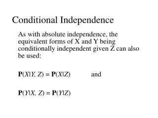
Conditional Independence. As with absolute independence, the equivalent forms of X and Y being conditionally independent given Z can also be used: P ( X|Y, Z ) = P ( X|Z ) and P ( Y|X, Z ) = P ( Y|Z ). Example of the Key Property. The following conditional independence holds:

Conditional Independence
E N D
Presentation Transcript
Conditional Independence • As with absolute independence, the equivalent forms of X and Y being conditionally independent given Z can also be used: P(X|Y, Z) = P(X|Z) and P(Y|X, Z) = P(Y|Z)
Example of the Key Property • The following conditional independence holds: P(MaryCalls |JohnCalls, Alarm, Earthquake, Burglary) = P(MaryCalls | Alarm)
Conditional Independence Again • A node X is conditionally independent of its non-descendants given Parents(X). • Markov Blanket of X: set consisting of the parents of X, the children of X, and the other parents of the children of X. • X is conditionally independent of all other nodes in the network given its Markov Blanket.
Representation Size • At first glance it would appear that the space to represent a Bayes Net is necessarily quadratic (possible number of arcs) in the number of random variables. • But recall we also must represent the CPT of each node, which in general will have size exponential in the number of parents of the node.
Representation Size • If we assume n boolean variables the network can be specified by n2k numbers in contrast to 2n for the joint. • For example: n=20 and each has at most k = 5, BN requires 640 numbers but the full joint needs over a million!
The Basic Inference Task in Bayesian Networks • Given some observed event (some assignment of values to a set of evidence variables), compute the posterior probability distribution over a set of query variables. • Variables that are neither evidence variables nor query variables are hidden variables. • Most common query: P(X|e).
Generality of Approach • A Bayes Net is flexible enough that any variable can be the query variables, and any variables can be evidence variables. • Algorithms we consider are easily extended to handle queries with multiple query variables.
Example Query • P(Burglary | JohnCalls=true, MaryCalls=true) = <0.284,0.716> • How can we compute such answers? • One approach is to compute entire full joint distribution represented by the network, and use our earlier algorithm. But this would defeat the entire purpose of Bayes Nets.
Inference By Enumeration • Recall the ENUMERATEJOINTASK procedure based on the preceding equation, which computed the answers to queries given the full joint represented as a table. • We will modify ENUMERATEJOINTASK to use the Bayes Net instead of the table. Need only get desired table entries using Bayes Net.
Getting a Full Joint Table Entry from a Bayes Net • Recall: • A table entry for X1 = x1,…,Xn = xn is simply P(x1,…,xn) which can be calculated based on the Bayes Net semantics above. • Therefore the CPTs provide a decomposed representation of the joint. • Recall example:
Example of Full Procedure • Query: P(Burglary | JohnCalls=true, MaryCalls=true) • P(B|j,m) = • Solve without the normalization constant for both B = true and B = false, and then compute the normalization constant and the final probabilities.
Example (Continued) Normalizing: a(0.000592 + 0.001494) = 1.0 a = 1.0/0.002086 = 479 P(B|j,m) = <0.284 , 0.716>

