Spatial STEM :

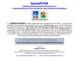
1. SpatialSTEM: A Mathematical/Statistical Framework for Understanding and Communicating Map Analysis and Modeling Part 3) Spatial Statistics. Spatial Statistics involves quantitative analysis of the “numerical context” of mapped data, such as characterizing the geographic distribution, relative comparisons, map similarity or correlation within and among data layers. Spatial Analysis and Spatial Statistics form a map-ematics that uses sequential processing of analytical operators to develop complex map analyses and models. Its approach is similar to traditional statistics except the variables are entire sets of geo-registered mapped data. Part 3) Spatial Statistics. Spatial Statistics involves quantitative analysis of the “numerical context” of mapped data, such as characterizing the geographic distribution, relative comparisons, map similarity or correlation within and among data layers. Spatial Analysis and Spatial Statistics form a map-ematics that uses sequential processing of analytical operators to develop complex map analyses and models. Its approach is similar to traditional statistics except the variables are entire sets of geo-registered mapped data. This PowerPoint with notes and online links to further reading is posted at www.innovativegis.com/basis/Courses/SpatialSTEM/Workshop/ Presented byJoseph K. Berry Adjunct Faculty in Geosciences, Department of Geography, University of Denver Adjunct Faculty in Natural Resources, Warner College of Natural Resources, Colorado State UniversityPrincipal, Berry & Associates // Spatial Information Systems Email: jberry@innovativegis.com— Website: www.innovativegis.com/basis

2. Thematic Mapping = Map Analysis (Average elevation by district) Thematic Mapping assigns a “typical value” to irregular geographic “puzzle pieces” (map features) describing the characteristics/condition without regard to their continuous spatial distribution (non-quantitative characterization) …average is assumed to be everywhere within each puzzle piece (+ Stdev) Worst “Thematic Mapping” (Discrete Spatial Object) Average Elevation of Districts 500 1539 2176 (0) Best (39) (9) 653 1099 (29) (21) … at least includeCoffVar in Thematic Mapping results 1779 (9) 1080 (24) (Berry)

3. Spatial Data Perspectives (numerically defining the What in “Where is What”) Numerical Data Perspective: how numbers are distributed in “Number Space” • Qualitative: deals with unmeasurable qualities(very few math/stat operations available) • Nominal numbers are independent of each other and do not imply ordering – like scattered pieces of wood on the ground 6 Nominal —Categories 4 5 5 2 4 1 • Ordinal numbers imply a definite ordering from small to large – like a ladder, however with varying spaces between rungs 3 2 6 3 Ordinal —Ordered 1 • Quantitative: deals with measurable quantities (a wealth of math/stat operations available) • Interval numbershave a definite ordering and a constant step – like a typical ladder with consistent spacing between rungs Interval —Constant Step 6 6 5 5 4 4 • Ratio numbers has all the properties of interval numbers plus a clear/constant definition of 0.0 – like a ladder with a fixed base. 3 3 Ratio —Fixed Zero 2 2 0 1 1 • Binary: a special type of number where the range is constrained to just two states— such as 1=forested, 0=non-forested Spatial Data Perspective: how numbers are distributed in “Geographic Space” • Choroplethnumbersform sharp/unpredictable boundaries in geographic space – e.g., a road “map” Elevation —Continuous gradient Roads —Discrete Groupings • Isoplethnumbers form continuous and often predictable gradients in geographic space–e.g., an elevation “surface” (Berry)

4. Overview of Map Analysis Approaches (Spatial Analysis and Spatial Statistics) Traditional GIS Forest Inventory Map • Points, Lines, Polygons • Discrete Objects • Mapping and Geo-query Spatial Statistics Traditional Statistics Spatial Distribution (Surface) Minimum= 5.4 ppm Maximum= 103.0 ppm Mean= 22.4 ppm StDEV= 15.5 • Mean, StDev (Normal Curve) • Central Tendency • Typical Response (scalar) • Map of Variance (gradient) • Spatial Distribution • Numerical Spatial Relationships Spatial Analysis Elevation (Surface) • Cells, Surfaces • Continuous Geographic Space • Contextual Spatial Relationships …last session (Berry)

5. Spatial Statistics Operations(Numerical Context) GIS as “Technical Tool” (Where is What) vs. “Analytical Tool” (Why, So What and What if) Map Stack Grid Layer Spatial Statistics Spatial Statisticsseeks to map the spatial variation in a data set instead of focusing on a single typical response (central tendency) ignoring the data’s spatial distribution/pattern, and thereby provides a mathematical/statistical framework for analyzing and modeling the Numerical Spatial Relationships within and among grid map layers Statistical Perspective: Basic Descriptive Statistics (Min, Max, Median, Mean, StDev, etc.) Basic Classification(Reclassify, Contouring, Normalization) Map Comparison (Joint Coincidence, Statistical Tests) Unique Map Statistics (Roving Window and Regional Summaries) Surface Modeling (Density Analysis, Spatial Interpolation) Advanced Classification (Map Similarity, Maximum Likelihood, Clustering) Predictive Statistics (Map Correlation/Regression, Data Mining Engines) Map Analysis Toolbox …let’s consider some examples (Berry)

6. Spatial Variable Dependence(the keystone concept in Spatial Statistics) There are two types of spatial dependency based on …“what occurs at a location in geographic space is related to” — 1) …the conditions of that variable at nearby locations, termed • Spatial Autocorrelation(intra-variable dependence; within a map layer) Surface Modeling – identifies the continuous spatial distribution implied in a set of discrete point samples Discrete Point Map Continuous Map Surface • 2) …the conditions of other variables at that location, termed Spatial Data Mining – investigates spatial relationships among multiple map layers by spatially evaluating traditional statistical procedures • Spatial Correlation (inter-variable dependence; among map layers) Map Stack – relationships among maps are investigated by aligning grid maps with a common configuration— same #cols/rows, cell size and geo-reference Data Shishkebab– within a statistical context, each map layer represents a Variable; each grid space a Case; and each value a Measurement …with all of the rights, privileges, and responsibilities of non-spatial mathematical, numerical and statistical analysis (Berry)

7. Desktop Mapping Data Space Field Data Map Analysis Geographic Space Standard Normal Curve Average = 22.0 StDev = 18.7 22.0 Desktop Mapping (GeoExploration) vs. Map Analysis (GeoScience) “Maps are numbers first, pictures later” — “Quantitative analysis of mapped data” Desktop Mappinggraphically links generalized statistics to discrete spatial objects (Points, Lines, Polygons)—spatially aggregated summaries (GeoExploration) X, Y, Value Point Sampled Data (Numeric Distribution) (Geographic Distribution) 40.7…not a problem Discrete Spatial Object Continuous Spatial Distribution High Pocket Spatially Generalized Spatially Detailed Discovery of sub-area… Adjacent Parcels Map Analysis map-ematically relates patterns within and among continuous spatial distributions (Map Surfaces)— spatially disaggregated analysis (GeoScience) (Berry)

8. Surface Modeling Approaches …spatial dependency within a single map layer (Spatial Autocorrelation) Surface Modelingidentifies the continuous spatial distribution implied in a set of discrete point data using one of four basic approaches— • Map Generalization“best fits” a polynomial equation to the entire set of geo-registered data values • Geometric Facets“best fits” a set of geometric shapes (e.g., irregularly sized/shaped triangles) to the data values • Density Analysis“counts or sums” data values occurring within a roving window(Qualitative/Quantitative) • Spatial Interpolation“weight-averages” data values within a roving window based on a mathematical relationship relating Data Variation to Data Distance that assumes “nearby things are more alike than distant things” (Quantitative)… 1 …Inverse Distance Weighted (IDW)interpolation uses a fixed 1/DPowerGeometric Equation …Kriginginterpolation uses a Derived Equation based on regional variable theory (Variogram) 0 …instead of a fixed geometric decay function, a data-drivencurve is derived 1 …and used to determine the sample weights used for interpolating each map location …inverse determines interpolation weights 0 (Berry)

9. Creating a Crime Risk Density Surface (Density Analysis) Density Analysis “counts or sums” data values within a specified distance from each map location (roving window) to generate a continuous surface identifying the relative spatial concentration of data within a project area, such as the number of customers or bird sightings within a half mile. Reclassify Geo-Coding Vector to Raster Grid Incident Counts Crime Incident Reports Crime Incident Locations Classified Crime Risk Roving Window Geo-codingidentifies geographic coordinates from street addresses Density Surface Totals Calculates the total number of reported crimes within a roving window– Density Surface Totals Grid Incident Countsthe number of incidences (points) within in each grid cell 91 3D surface plot 2D perspective display of crime density contours 2D display of discrete Grid Incident Counts Classified Crime Risk Map (Berry)

10. Spatial Interpolation (iteratively smoothing the spatial variability) The iterative smoothing process is similar to slapping a big chunk of modeler’s clay over the “data spikes,” then taking a knife and cutting away the excess to leave a continuous surface that encapsulates the peaks and valleys implied in the original data Data Location Data Table Continuous Surface Non-sampled locations in the analysis frame are assigned the value ofthe closest sampled location… …the “abrupt edges” forming the blocks are iteratively smoothed (local average)… (Geo-tagged Data Set) Discrete Point Data Iteration #1 Iteration #2 Iteration #3 Nearest Neighbor Valuable insight into the spatial distribution of the field samples is gained by comparing the “response surface” with the arithmetic average… Average value = 23 (+ 26) …for each location, its locally implied response is compared to the generalized average Iteration #4 Iteration #9 Iteration #19 Iteration #29 Iteration #39 Iteration #49 Iteration #69 Iteration #99 (digital slide show SStat2) (Berry)

11. Assessing Interpolation Results (Residual Analysis) The difference between an actual value (measured) and an interpolated value (estimated) is termed the Residual. The residuals can be summarized to assess the performance of different interpolation techniques… …with the best map surface as the one that has the “best guesses” (interpolated estimates) Actual – Estimate = Residual 23 – 0 = 23 Bad Guess Best Surface (Berry)

12. Spatial Variable Dependence(the keystone concept in Spatial Statistics) There are two types of spatial dependency based on …“what occurs at a location in geographic space is related to” — 1) …the conditions of that variable at nearby locations, termed • Spatial Autocorrelation(intra-variable dependence; within a map layer) Surface Modeling – within a map layer (Spatial Autocorrelation) …deriving the Spatial Distribution Surface Modeling – identifies the continuous spatial distribution implied in a set of discrete point samples Discrete Point Map Continuous Map Surface • 2) …the conditions of other variables at that location, termed Spatial Data Mining – investigates spatial relationships among multiple map layers by spatially evaluating traditional statistical procedures • Spatial Correlation (inter-variable dependence; among map layers) Map Stack – relationships among maps are investigated by aligning grid maps with a common configuration— same #cols/rows, cell size and geo-reference Data Shishkebab– within a statistical context, each map layer represents a Variable; each grid space a Case; and each value a Measurement …with all of the rights, privileges, and responsibilities of non-spatial mathematical, numerical and statistical analysis (Berry)

13. Yield Monitor GPS Map Comparison (spatially evaluating the T-test) Cell-by-cell paired values are subtracted Spatially Evaluating the “T-Test” The T-statistic equation is evaluated by first calculating a map of the Difference(Step 1) and then calculating maps of the Mean(Step 2) and Standard Deviation(Step 3) of the Difference within a “roving window.” The T-statistic is calculated using the derived Mean and StDev maps of the localized difference using the equation (step 4) — spatially localized solution “On-the-Fly” yield map records both the Numeric and Spatial distributions Precision Agriculture Step 4. Calculate the “Localized” T-statistic (using a 5-cell roving window)for each grid cell location Traditional Agriculture Research Numeric Distribution Sample Plots Geo-registered Grid Map Layers Discrete point data assumed to be spatially independent 5-cell radius “roving window” …containing 73 paired values that are summarized and assigned to center cell Spatial Distribution T_test …the result is map of the T-statistic indicating how different the two map variables are throughout geographic space and a T-test map indicating where they are significantly different. Col 33 T_statistic Evaluate the Map Analysis Equation Row 53 (Berry)

14. Map Similarity (identifying similar numeric patterns) Geographic Space— relative spatial position of map values Locations identical to the Comparison Point are set to 100% similar (Identical numerical pattern) The farthest away point in data space is set to 0 (Least Similar numerical pattern) Data Space— relative Numerical magnitude of map values …all other Data Distances are scaled in terms of their relative similarity to the comparison point (0 to 100% similar) Farthest away Map Stack Each “floating ball” in the Data Space scatter plot schematically represents a location in the field (Geographic Space). The position of a ball in the plot identifies the relative phosphorous (P), potassium (K) and nitrogen (N) levels at that location. (Berry)

15. Clustering (automated map similarity) …clusters of “floating balls” in data space identify locations in the field with similar data patterns – Data Zones (groupings of locations having similar data patterns) Cyber-Farmer, Circa 1992 …fertilization rates vary “on-the-fly” for the different clusters Variable Rate Application (Berry)

16. Predictive Spatial Statistics (map regression) Map regression measures of the association between one map variable (dependent variable) and one or more other map variables (independent variables) expressing the relationship as a predictive equation that can be applied to other data sets …pass map layers to any Statistics or Data Mining package Spatial DBMS — export grid layers to dB with each cell a record & each layer a field For example, predicting Loan Concentration based on Housing Density, Home Value and Home Age in a city Univariate Linear Regressions Dependent Mapvariable is what you want to predict… Multivariate Linear Regression Error = Predicted – Actual …substantially under-estimates (but 2/3 of the error within 5.26 and 16.94) …can use error to generate Error Ranges for calculating new regression equations …from a set of easily measured Independent Map variables Stratified Error Actual Predicted Error Surface (Berry)

17. Spatial Statistics Operations(Numerical Context) GIS as “Technical Tool” (Where is What) vs. “Analytical Tool” (Why, So What and What if) Map Stack Grid Layer Spatial Statistics Spatial Statisticsseeks to map the spatial variation in a data set instead of focusing on a single typical response (central tendency) ignoring the data’s spatial distribution/pattern, and thereby provides a mathematical/statistical framework for analyzing and modeling the Numerical Spatial Relationships within and among grid map layers Statistical Perspective: …discussion focused on these groups of spatial statistics — see reading references for more information on all of the operations Basic Descriptive Statistics (Min, Max, Median, Mean, StDev, etc.) Basic Classification(Reclassify, Contouring, Normalization) Map Comparison (Joint Coincidence, Statistical Tests) Unique Map Statistics (Roving Window and Regional Summaries) Surface Modeling (Density Analysis, Spatial Interpolation) Advanced Classification (Map Similarity, Maximum Likelihood, Clustering) Predictive Statistics (Map Correlation/Regression, Data Mining Engines) Map Analysis Toolbox (Berry)