Chapter 4. Random Processes
Chapter 4. Random Processes. 4.1 Introduction 1. Deterministic signals: the class of signals that may be modeled as completely specified functions of time. 2. Random signals: it is not possible to predict its precise value in advance. ex) thermal noise

Chapter 4. Random Processes
E N D
Presentation Transcript
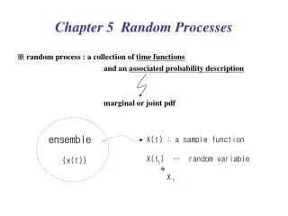
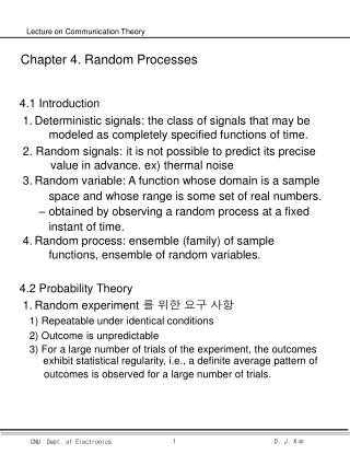
Chapter 4. Random Processes • 4.1 Introduction • 1. Deterministic signals: the class of signals that may be modeled as completely specified functions of time. • 2. Random signals: it is not possible to predict its precise value in advance. ex) thermal noise • 3. Random variable: A function whose domain is a sample • space and whose range is some set of real numbers. • – obtained by observing a random process at a fixed • instant of time. • 4. Random process: ensemble (family) of sample • functions, ensemble of random variables. • 4.2 Probability Theory • 1. Random experiment 를 위한 요구 사항 • 1) Repeatable under identical conditions • 2) Outcome is unpredictable • 3) For a large number of trials of the experiment, the outcomes exhibit statistical regularity, i.e., a definite average pattern of • outcomes is observed for a large number of trials.
2. Relative-Frequency Approach • 1) Relative frequency • 2) Statistical regularity Probability of event A. • 3. Axioms of Probability. • 1) 용어 a) Sample points sk: kth outcome of experiment b) Sample space S: totality of sample points c) Sure event: entire sample space S d) : null or impossible event e) Elementary event: a single sample point • 2) Definition of probability a) A sample space S of elementary events b) A class of events that are subsets of S. c) A probability measure P() assigned to each event A in the class , which has the following properties: Axioms of Probability
1-p A0 [0] B0 [0] p p [1] A1 B1 [1] 1-p • 3) Property 1. • 4) Property 2. If M mutually the exclusive events have the exclusive property then • 5) Property 3. • 4. Conditional Probability • 1) Conditional Probability of given A (given A means that event A has occurred) • 2) Statistically independent ex1) BSC (Binary Symmetric Channel) • Discrete memoryless channel
Priori prob. Conditional prob. or likelihood [0]송신[1]수신확률 [0]송신[0]수신확률 Output prob. Posteriori prob. [0]수신[0]송신확률 [1]수신[1]송신확률 4.3 Random variables 1.개요 1) Random variable: A function whose domain is a sample space and whose range is some set of real numbers 2) Discrete r. v. : X(k), k번째 sample ex)주사위 range {1,,6} Continuous r. v. : X ex) 8시~ 8시 10분 버스도착시간 3) Cumulative distribution function (cdf) or distribution fct. FX(x) = P(X x) a) 0 FX(x) 1 b) if x1 < x2, FX(x1) FX(x2), monotone-nondecreasing fct. • .
4) pdf (probability density fct.) • pdf: nonnegative fct., total area = 1 • ex2)
2. Several random variables (2 random variables) • 1) Joint distribution fct. • 2) Joint pdf • 3) Total area • 4) Conditional prob. density fct. (given that X = fixed x) • If X,Y are statistically independent • fY(y|x) = fY(y) • Statistically independent fX,Y(x,y) = fX(x)fY(y) • 4.4 Statistical Average • 1. Mean or expected value • 1) Continuous • ex) 0 10
2) Discrete • 2. Function of r. v. • Y=g(X) X, Y : r. v. • 3. Moments • 1) n-th moments • 2) Central moments • where is standard deviation
; Chebyshev inequality • X2의 meaning: randomness, effective width of fX(x) • 그 이유는 Chebyshev inequality을 통해서 알 수 있다. • 4. Characteristic function • Characteristic function X(v) fX(x) • ex4) Gaussian Random Variable
O X • 5. Joint moments E[X] = 0 or E[Y] = 0 X, Y are orthogonal X, Y are statistically independent uncorrelated uncorrelated
Y y X x • 4.5 Transformations of Random variables: Y=g(X) • 1. Monotone transformations: one-to-one • 2. Many-to-one transformations • where xk = solution of g(x) = y
4.6 Random processes or schocastic process • r. v. {X}: Outcomes of a random experiment is mapped into a number • r. p. {X(t)} or {X(t,s)}: Outcomes of a random experiment is mapped into a waveform that is fct. of time indexed ensemble (family) of r. v. • Sample function xj(t) = X(t,sj) {x1(t),x2(t),,xn(t)} • {x1(tk),x2(tk),xn(tk)} = {X(tk,s1),X(tk,s2)X(tk,sn)} constitutes a random variable • r. p. 의 예) X(t) = A cos (2fct+), Random Binary Wave, gaussian noise sample space
4.7 Stationary • 1. r. p. X(t) is stationary in the strict sense – If for all time shift , all k and all possible t1,,tk. • < observation > • 1) k = 1, FX(t)(x) = FX(t+)(x) = FX(x) for all t & . 1st order distribution fct. of a stationary r. p. is independent of time • 2) k = 2 & = -t, for all t1& t2 • 2nd order distribution fct. of a stationary r. p. depends only • on the differences between the observation time • 2. Two r. p. X(t),Y(t) are jointly stationary if the joint • distribution functions of r. v. X(t1),,X(tk) and Y(t1’), • ,Y(tk’) are invariant with respect to the location of the • origin t = 0 for all k and j, and all choices of observation • times t1,,tk and t1’, ,tk’. • ex6)
probability of the joint event • A={ai < X(ti) bi} i=1, 2, 3 • 4.8 Mean, Correlation, and Covariance functions • 1. Mean of r. p. • For stationary r. p. constant, for all t • 2. Autocorrelation fct. of r. p. X(t) • For stationary r. p. RX(t1,t2) = RX(t2-t1)
o x • 3. Autocovariance fct. of stationary r. p. X(t) CX(t1,t2)=E[(X(t1) - X)(X(t2) -X)] =RX(t2 - t1) - X2 • 4. Wide-sense stationary • strict-sense stationary wide sense stationary • 5. Properties of the Autocorrelation Function • Autocorrelation fct. of stationary process X(t) RX()=E[X(t+)X(t)] for all t • Properties a) Mean-square value by setting = 0 RX(0) = E[X2(t)] b) RX(): even fct. RX() = RX(-) c) RX() has its maximum at = 0, RX() RX(0) pf. of c)
Physical meaning of RX() • “Interdependence “ of X(t) and X(t+) • Decorrelation time 0: for > 0, RX() < 0.01RX(0) ex7) Sinusoidal wave with Random phase
ex8) Random Binary Wave • RX(0) = E[X(t)X(t)] = A2 • RX(T) = E[X(t)X(t+T)] = 0
6. Cross-correlation Functions • r. p. X(t) with RX(t,u) • r. p. Y(t) with autocorrelation RY(t,u) • Cross-correlation fct. of X(t) and Y(t) • RXY(t,u) = E[X(t)Y(u)] • RYX(t,u) = E[Y(t)X(u)] • Correlation Matrix of r. p. X(t) and Y(t) • If X(t) and Y(t) are each w. s. s. and jointly w. s. s. • where = t-u • 여기서 RXY() RXY(-) i.e. not even fct. • RXY(0) is not maximum • RXY() = RYX(-)
ex9) Quadrature - Modulated Processes • X1(t) and X2(t) from w. s. s. r. p. X(t) • X1(t)=X(t)cos(2fct + ) • X2(t)=X(t)sin(2fct + ) where • is independent of X(t) • Cross-correlation fct. • R12() = E[X1(t)X2(t-)] • = E[X1(t)X2(t-)]E[cos(2fct+)sin(2f1t-2fc+)] • = • R12(0)=E[X1(t)X2(t)]=0 orthogonal • 4.9 Ergodicity • For sample function x(t) of w. s. s. r. p. x(t) with -T t T • – Time average (dc value)
– Mean of time average X(T) • 1. w. s. s. r. p. X(t) is ergodic in the mean • 2. w. s. s. r. p. X(t) is ergodic in the autocorrelation fct. where RX(,T) = = time averaged autocorrelation fct. of sample fct. x(t) from w. s. s. r. p. x(t) • 4.10 Transmission of a r. p. through a linear filter Thus 구해보면 w.s.s r.p w.s.s r.p 구할 수 없다
1. Mean of Y(t) • 2. Autocorrelation fct. • Mean square value E[Y2(t)]=RY(0)
4.11 Power Spectral density • 1. Mean square value of Y(t)를 p. s. d. 로 표현 • h1(1) H(f) • Power spectral density or power spectrum of w. s. s. r. v. X(t) • Mean square value of Y(t)
2. Properties of the Power Spectral Density • 1) Einstein - Wiener- Khintchine relations • 2) Property 1. • For w. s. s. r. p., • 3) Property 2. • Mean square value of w. s. s. r. p. • 4) Property 3. • For w. s. s. r. p., SX(f) 0 for all f. • 5) Property 4. • SX(-f) = SX(f): even fct. • RX(-) = RX() • 6) Property 5. The p. s. d., appropriately normalized, has the properties usually associated with a probability density fct. • 7) rms bandwidth of w. s. s. r. p. X(t)
ex10) Sinusoidal wave with Random Phase R. p. X(t) = A cos (2fC(t) + ) where is uniform r. v. over [-, ] ex11) Random Binary wave with +A & -A
Energy spectral density of a rectangular pulse g(t) ex12) Mixing of a r. p. with a sinusoidal process. • 3. Relation among the Power Spectral Density of the Input • and Output Random Process
ex13) Comb filter differentiator
4. Relation among the Power Spectral Density and the • Amplitude Spectrum of a Sample Function Sample fct. x(t) of w. s. s. & ergodic r. p. X(t) with SX(f) X(f,T): FT of truncated sample fct. x(t) Conclusion) Sample function 으로부터 SX(f)를 구할 수 있다. • 5. Cross Spectral Density A measure of the freq. interrelationship between 2 random process
X(t) V(t) h1(t) Y(t) h2(t) Z(t) ex14) – X(t) and Y(t) has zero mean, w. s. s. r. p. – Consider Z(t) = X(t)+Y(t) – Auto correlation of Z(t) ex15) X(t), Y(t); Jointly w. s. s. r. p. where h1, h2 are stable, linear, time-invariant filter Cross correlation fct. of V(t) and Z(t)
4.12 Gaussian Process • 1. Definition Process X(t) is a Gaussian process if every linear functional of X(t) is a Gaussian r. v. If the r. v. Y is a Gaussian distributed r. v. for every g(t), then X(t) is a Gaussian process 여기서
2. Virtues of Gaussian process • 1) Gaussian process has many properties that make analytic results possible • 2) Random processes produced by physical phenomena are often such that a Gaussian model is appropriate. • 3. Central Limit Theorem • 1) Let Xi, I = 1, 2, , N be a set of r. v. that satisfies a) The Xi are statistically independent b) The Xi have the same p. d. f. with mean X and variance X2 Xi : set of independently and identically distributed (i. i. d.) r. vs. • Now Normalized r. v. < Central limit theorem > The probability distribution of VN approaches a normalized Gaussian distribution N(0,1) in the limit as N approaches infinity. 즉 Normalized r. v. 이 많이 모여서 하나의 r. v. 을 만들면 이는 N(0,1) 이 된다.
Gaussian P. Gaussian P. stable, linear • 4. Properties of Gaussian Process • 1) Property 1. • X(t) h(t) Y(t) If a Gaussian process X(t) is applied to a stable linear filter, then the random process Y(t) developed at the output of the filter is also Gaussian. • 2) Property 2. Consider the set of r. v. or samples X(t1), X(t2), , X(tn) obtained by observing a r. p. X(t) at times t1, t2,, tn. If the process X(t) is Gaussian, then this set of r. vs. are jointly Gaussian for any n, with their n-fold joint p. d. f. being completely determined by specifying the set of means and the set of auto covariance functions • 3) Property 3. If random variables X(t1), X(t2), , X(tn) from Gaussian process X(t) are uncorrelated, i. e. then these random variables are statistically independent • 4.13 Noise • External: e. g. atmospheric, galactic, man-made noise • Internal: e. g. spontaneous fluctuation of I or V in electric circuits shot, themal noise
Channel Test Model < H. W > Chap 4, 4.6, 4.15, 4.23