Visible Surface Determination (VSD)

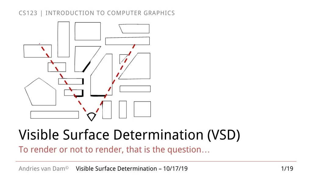
1. Visible Surface Determination (VSD) To render or not to render, that is the question… Visible Surface Determination – 10/17/19

2. What is it? • Given a set of 3-D objects and a view specification (camera), determine which edges or surfaces of the object are visible • why might objects not be visible? occlusion vs. clipping • clipping works on the object level (clip against view volume) • occlusion works on the scene level (compare depth of object/edges/pixels against other objects/edges/pixels) • Also called Hidden Surface Removal (HSR) • We begin with some history of previously used VSD algorithms Visible Surface Determination – 10/17/19

3. Object-Precision Algorithms • Roberts ’63 - hidden line (edge) removal • Compare each edge with every object - eliminate occluded edges or parts of edges. • Complexity: since each object must be compared with all edges • A similar approach for hidden surfaces: • Each polygon is clipped by the projections of all other polygons in front of it • Invisible (occluded) surfaces are eliminated and visible sub-polygons are created • SLOW, ugly special cases, polygons only • Sutherland categorized algorithms according to whether they work on objects in the world (object precision) or with projections of objects in screen coordinates (image precision) and refer back to the world when z is needed Visible Surface Determination – 10/17/19

4. Painter’s Algorithm – Image Precision • Back-to-front algorithm was used in the first hardware-rendered scene, the 1967 GE Flight Simulator by Schumacher et al using a video drum to hold the scene • http://www.youtube.com/watch?v=vajvwNctrb8 • Create drawing order so each polygon overwrites the previous one. This guarantees correct visibility at any pixel resolution • Work back to front; find a way to sort polygons by depth (z), then draw them in that order • do a rough sort of polygons by smallest (farthest) z-coordinate in each polygon • scan-convert most distant polygon first, then work forward towards viewpoint (“painters’ algorithm”) • See 3D depth-sort algorithm by Newell, Newell, and Sancha • https://en.wikipedia.org/wiki/Newell%27s_algorithm • Can this back-to-front strategy always be done? • problem: two polygons partially occluding each other – need to split polygons, very messy • the principle is still relevant today for transparent polygons • Comparison of algorithms Interlocking polygons can cause the Painter’s Algorithm to fail Visible Surface Determination – 10/17/19

5. Clicker Visible Surface Determination – 10/17/19

6. Depth sorting for transparency https://hub.jmonkeyengine.org/t/alpha-transparency-sorting-your-z-buffer-and-you/33709 Visible Surface Determination – 10/17/19 • Alpha compositing is a simple case of Porter-Duff compositing • https://en.wikipedia.org/wiki/Alpha_compositing • First, render all opaque objects • Then, render transparent objects back-to-front • Again, can run into complications if transparent polygons are not all sortable… • Transparency is tricky to get right in all cases in a rasterization-based renderer • Z-buffer’s advantage is no need for sorting, so sorting adds complexity • Trivial for raytracing, though!

7. Hardware Polygon Scan Conversion: VSD (1/4) Perform backface culling • If normal is facing in same direction as LOS (line of sight), it’s a back face: • if , then polygon is invisible – discard • if , then polygon may be visible (if not, occluded) 1 2 +y (-1, 1, -1) +z +x (1, -1, 0) Canonical perspective-transformed view volume with cube 3 Finally, clip against normalized view volume (-1 < x < 1), (-1 < y < 1), (-1 < z < 0) Visible Surface Determination – 10/17/19

8. Backface culling assumes objects are closed No Backface culling With Backface culling https://en.wikipedia.org/wiki/Back-face_culling Visible Surface Determination – 10/17/19 • A triangle facing away from you is only guaranteed to be invisible if there’s something else in front of. • This is only guaranteed for closed, solid objects (e.g. a sphere) • Objects with ‘holes’ may expose back-facing triangles to the viewer; backface culling results in errors (see skulls on right) • OpenGL allows you to toggle backface culling • glEnable(GL_CULL_FACE)

9. Hardware Polygon Scan Conversion: VSD (2/4) • Still need to determine object occlusion (point-by-point) • How to determine which point is closest? • i.e. is closer than • In perspective view volume, have to compute projector and which point is closest along that projector – no projectors are parallel • Perspective transformation causes all projectors to become parallel • Simplifies depth comparison to z-comparison • The Z-Buffer Algorithm: • Z-buffer has scalar value for each screen pixel, initialized to far plane’s z (maximum) • As each object is rendered, z value of each of its sample points is compared to z value in the same (x, y) location in z-buffer • If new point’s z value less than or equal to previous one (i.e., closer to eye), its z-value is placed in the z-buffer and its color is placed in the frame buffer at the same (x, y); otherwise previous z value and frame buffer color are unchanged • Can store depth as integers or floats – z-compression a problem either way (see Viewing III44-46) • Integer still used in OGL Visible Surface Determination – 10/17/19

10. Z-Buffer Algorithm void zBuffer(){ int x, y; for(y =0; y < YMAX; y++) for(x =0; x < XMAX; x++){ WritePixel(x, y, BACKGROUND_VALUE); WriteZ(x, y,1); } for each polygon { for each pixel in polygon’s projection { //plane equation double pz = Z-value at pixel (x, y); if(pz <= ReadZ (x, y)){ // New point is closer to front of view WritePixel(x, y, color at pixel (x, y)) WriteZ (x, y, pz); } } } } • Draw every polygon that we can’t reject trivially (totally outside view volume) • If we find a piece (one or more pixels) of a polygon that is closer to the front than what was painted there before, we paint over whatever was there before • Use plane equation for polygon,        z = f(x, y) • Note: use positive z here [0, 1] Visible Surface Determination – 10/17/19

11. Hardware Scan Conversion: VSD (3/4) • Requires two “buffers” • Intensity Buffer: our familiar RGB pixel buffer, initialized to background color • Depth (“Z”) Buffer: depth of scene at each pixel, initialized to 255 • Polygons are scan-converted in arbitrary order. When pixels overlap, use Z-buffer to decide which polygon “gets” that pixel + = integer Z-buffer with near = 0, far = 255 + = Visible Surface Determination – 10/17/19 https://en.wikipedia.org/wiki/Z-buffering

12. Hardware Scan Conversion: VSD (4/4) • After scene gets projected onto film plane we know depths only at locations in our depth buffer that our vertices got mapped to • So how do we efficiently fill in all the “in between” z-buffer information? • Simple answer: incrementally! • Remember scan conversion/polygon filling? As we move along Y-axis, track x position where each edge intersects scan line • Do the same for z coordinate with y-z slope instead of y-x slope • Knowing z1, z2, and z3 we can calculate za and zb for each edge, and then incrementally calculate zp as we scan. • Similar to interpolation to calculate color per pixel (Gouraud shading) • Barycentric interpolation also works (triple-interpolation is more efficient than multiple pair-wise interpolations) Visible Surface Determination – 10/17/19

13. Advantages of Z-buffer • Dirt-cheap and fast to implement in hardware, despite brute force nature and potentially many passes over each pixel • Requires no pre-processing, polygons can be treated in any order! • Allows incremental additions to image – store both frame buffer and z-buffer and scan-convert the new polygons • Lost coherence/polygon id’s for each pixel, so can’t do incremental deletes of obsolete information. • Technique extends to other surface descriptions that have (relatively) cheap z= f(x, y) computations (preferably incremental) Visible Surface Determination – 10/17/19

14. Review of “Unhinging” Perspective Transformation • The perspective transformation maps the 2-unit perspective frustum to the 2-unit cuboid parallel view volume (x,y dimensions, 1 in z) • The far plane square cross-section stays fixed at z = -1 and the near plane  cross-section at z = - near/far moves to z = 0 • Where is the “hinge”? The apex/CoP is at (0, 0, 0) – consider pulling a “pin” out of this shared vertex so that the sides of the frustum can rotate about axes at the corners at z = -1 to make the shared vertices move to (±1, ±1, 0) and the planes move from 45° to 90°. Visible Surface Determination – 10/17/19

15. -x +x near Disadvantages of Z-Buffer Before perspective: • Perspective foreshortening (see slides 44-46 in Viewing III) • Compression in z-axis in post-perspective space • Objects far away from camera have z-values very close to each other • Depth information loses precision rapidly • Leads to z-ordering bugs called z-fighting far -z +x -x near After perspective: far Visible Surface Determination – 10/17/19 -z

16. Z-Fighting (1/4) • Z-fighting occurs when two primitives have similar values in the z-buffer • Coplanar polygons not axis-aligned (two polygons that occupy the same space) • One is arbitrarily chosen over the other, but z varies across the polygons and binning will cause artifacts, as shown on next slide • Behavior is deterministic: the same camera position gives the same z-fighting pattern Two intersecting cubes Visible Surface Determination – 10/17/19

17. Z-Fighting (2/4) • Examples • /course/cs123/data/scenes/contest/ntom.xml: • https://youtu.be/9AcCrF_nX-I?t=8m10s (starting at 8:10) Visible Surface Determination – 10/17/19

18. Z-Fighting (3/4) Eye at origin, Looking down Z axis Blue, which is drawn after red, ends up in front of red 1 Red in front of blue 1 Overwrite if value in current z-value value in z-buffer x axis of image (each column is a pixel) Here the red and blue lines represent rasterized cross-sections of the red and blue coplanar polygons from the previous slide z-value bins Visible Surface Determination – 10/17/19

19. Z-Fighting (4/4) pull in • What if overwrite only if z-value is current value in buffer? • The same problem will occur if the red polygon is drawn after the blue. • What to do… • To mitigate z-fighting, we can increase the precision of the depth buffer, and decrease the ratio push out • Pull the far plane in, and push near plane out • Bound the relevant part of the scene as tightly as possible • Don’t want near plane too close to the eye • Use texture maps for small far away detail • If the ratio is too large, then perspective transformation more likely to map large z-values to the same bin • Huge range has to be mapped to , further z-values in camera-space given very little of this range, squashed severely • Objects will small z-values are blown up, given a huge amount of this range (think of how distorted objects get when placed next to your eye) • Affects the homogenized after projection (c = -near/far), very close to -1 for large z Visible Surface Determination – 10/17/19