In this module we will model: Electronic autowasher bias spring problems
340 likes | 516 Views
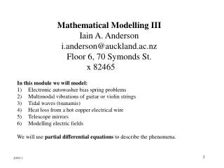
Mathematical Modelling III Iain A. Anderson i.anderson@auckland.ac.nz Floor 6, 70 Symonds St. x 82465 . In this module we will model: Electronic autowasher bias spring problems Multimodal vibrations of guitar or violin strings Tidal waves (tsunamis) Heat loss from a hot copper electrical wire

In this module we will model: Electronic autowasher bias spring problems
E N D
Presentation Transcript
Mathematical Modelling IIIIain A. Andersoni.anderson@auckland.ac.nzFloor 6, 70 Symonds St.x 82465 • In this module we will model: • Electronic autowasher bias spring problems • Multimodal vibrations of guitar or violin strings • Tidal waves (tsunamis) • Heat loss from a hot copper electrical wire • Telescope mirrors • Modelling electric fields • We will use partial differential equations to describe the phenomena. 2003/ 1
What are partial differential equations? Compare them with ordinary differential equations: In ODEs the unknown(s) depend(s) on one variable: In PDEs the unknown(s) depend(s) on more than one variable. PDEs contain partial derivatives. Here, T is the dependent variable and x and t the independent variables. The “” indicates that these are partial derivatives. There are more variables than one. In this case we have x and t
PDE’s can be used for modelling electric, magnetic, structural mechanical, thermodynamic and fluid dynamic phenomena.PDE’s relate space (x,y,z) and time (t) derivatives. Partial derivatives can represent velocities acceleration, forces, friction, heat gradients etc. The equation on the right is used for describing the flow of heat.
It is often useful to perform a few calculations using simple engineering models based on pde’s. These models will provide enough information to establish the feasibility of a design concept, troubleshoot a problem or select a construction material. • Basic steps of problem formulation and solution: • Model the problem and find an equation • Derive a solution to the equation • Fit the solution to the boundary conditions • Fit the solution to the initial conditions
Inner bowl Outer bowl GE dc brushless motor Suspension rod Bias spring Model 1: Troublesome electronic autowasher spring vibrations Bias spring resonance problems encountered during the development of the suspension for the F&P electronic autowasher “Gentle Annie” (1985). At 1100 rpm when the washing machine was in spin mode the bias spring would vibrate wildly and make contact with the pulley. Schematic of autowasher
Step 1: Model the problem and find an equationThe spring was long and slender like an elastic string. I recalled something I had learned in Engineering Mathematics II (The predecessor of MM3): How to derive the equation governing small transverse vibrations of an elastic string that is stretched to length L and then fixed at its endpoints. L
Assumptions:Mass per unit length is constant.Gravity can be neglectedMotion is in one plane
T2 Q P T1 Q P L x x+x Modelling the spring as an elastic string. Consider a “free body diagram” of a string segment: forces at ends = massacceleration
T2 Q P T1 forces at ends = massacceleration Now consider the forces acting on this string segment. We will find the deflection u(x,t) at any point x and t > 0. Note: ρ = linear density of string. Horizontal direction: (1) Vertical direction: (2)
T2 Q P T1 Divide equation 2 by equation 1 to get equation 3: (2) (1) (3) Note that tan = string slope at x and tan = string slope at x+Δx
x tan= string slope at x andtan = string slope at x+Δx Thus (4) After dividing eqn.3 by Tx, and substituting eqn.’s 4 for the tan functions, we have:
x Now let x0 x x+x
By letting Δx 0, we have obtained the one-dimensional wave equation: Rearrange and set c2 = T/ρ: (5) How do we obtain a solution for the autowasher spring?
Step 2: The solution We must find a solution that: Solves the equation andhas the potential to give useful results. Lets try a couple of trial solutions: u = C where C is a constant. 0 0
u = C works but this solution isn’t very useful. We want a solution that changes with time and that can be used for describing a moving spring. Lets try u = D x/t where D is another constant. -2D x/t3 0 This won’t satisfy the equation!
Instead of guessing we could start looking for a solution by making the assumption that it will be some function of x multiplied by a function of t: We obtain the solution using the method of “Separation of Variables”.
Separation of variables Substitute the solution u=X(x)T(t) into eqn. 5: (5) You get:
Now separate variables (get everything that’s a function of x on one side and everything that’s a function of t on the other):
Both sides are equal to a constant. Call it k: We get the two equations: Time (t) only Distance (x) only
Choose a sign for the constant that will give you sensible results. k should be negative. k=-2 . You now get 2 differential equations: (6)
Solutions to T and X are: (7) Demonstrate to yourself that the two expressions (eqn.’s 7) are solutions to eqn.’s 6.
The solution for u(x,t) equals X times T: (8) This looks OK. The sinusoidal terms will be useful for fitting a solution within the fixed length L. Prove that this solution satisfies the differential equation.
We must now find values for the constants A-D and λ. (8) Step 3: Fit the solution to the boundary conditions What boundary conditions would we use? The spring is tethered at the ends.
L Boundary conditions At x=0 u(0,t) = 0 Thus B= 0
At x=L u(L,t) = 0 So sin(L) = 0 or L = nπwhere n= 0,1,2,3,…. so or (9) n= 1,2,3,…. Note n=0 gives u0 =0
u1(x,t) 1st string mode Modeshape Nat. frequency
u2(x,t) 2nd string mode
u3(x,t) 3rd string mode
u1(x,t) The observed pattern of vibration for the bias spring resembled mode #1 The natural frequency is (Radians per second): Note: frequency in Hz can be obtained by dividing this by 2π.
ConclusionsMeasurements of T, ρ (mass per unit length), and Lfrom the bias spring confirmed that it would be resonant at ω1 = 115 radians/sec. This is equivalent to 18.3 Hz or 1100 rpm! The spring was de-tuned by careful redesign, to give it a lower linear density (mass per coil) so that its first mode would have a safe high resonant frequency of 146 radians/sec (1400rpm). Note that this wasn’t easy. Other factors had to be taken into account associated with the required spring stiffness and strength.