Download
1 / 35
350 likes | 452 Views
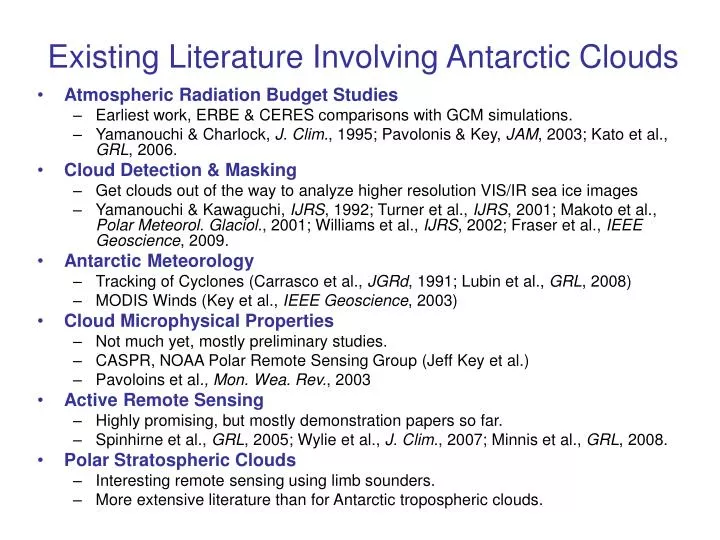
Existing Literature Involving Antarctic Clouds. Atmospheric Radiation Budget Studies Earliest work, ERBE & CERES comparisons with GCM simulations. Yamanouchi & Charlock, J. Clim. , 1995; Pavolonis & Key, JAM , 2003; Kato et al., GRL , 2006. Cloud Detection & Masking

E N D
Existing Literature Involving Antarctic Clouds • Atmospheric Radiation Budget Studies • Earliest work, ERBE & CERES comparisons with GCM simulations. • Yamanouchi & Charlock, J. Clim., 1995; Pavolonis & Key, JAM, 2003; Kato et al., GRL, 2006. • Cloud Detection & Masking • Get clouds out of the way to analyze higher resolution VIS/IR sea ice images • Yamanouchi & Kawaguchi, IJRS, 1992; Turner et al., IJRS, 2001; Makoto et al., Polar Meteorol. Glaciol., 2001; Williams et al., IJRS, 2002; Fraser et al., IEEE Geoscience, 2009. • Antarctic Meteorology • Tracking of Cyclones (Carrasco et al., JGRd, 1991; Lubin et al., GRL, 2008) • MODIS Winds (Key et al., IEEE Geoscience, 2003) • Cloud Microphysical Properties • Not much yet, mostly preliminary studies. • CASPR, NOAA Polar Remote Sensing Group (Jeff Key et al.) • Pavoloins et al., Mon. Wea. Rev., 2003 • Active Remote Sensing • Highly promising, but mostly demonstration papers so far. • Spinhirne et al., GRL, 2005; Wylie et al., J. Clim., 2007; Minnis et al., GRL, 2008. • Polar Stratospheric Clouds • Interesting remote sensing using limb sounders. • More extensive literature than for Antarctic tropospheric clouds.
Illustration of the Antarctic Cloud Detection Problem and Multispectral Solution (e.g., Yamanouchi & Kawaguchi, IJRS, 1992) Left: NOAA-14 AVHRR channel 1 image over part of West Antarctica at 2017 UTC on 1 December 1997. Right: Image of the brightness temperature difference between channels 3 and 4.
Scatter diagrams of the brightness temperature differences (A) channel 3 and channel 4, (B) channel 4 and channel 5, versus the channel 4 brightness temperature. Crosses refer to measurements north of -73oS. Circles refer to measurements between -73oS and -74oS. Squares refer to measurements below -76oS.
Scatter diagrams of the brightness temperature differences (A) channel 3 and channel 4, (B) channel 4 and channel 5, versus the channel 4 brightness temperature. Crosses refer to measurements north of -73oS. Circles refer to measurements between -73oS and -74oS. Squares refer to measurements below -76oS.
Cloud Microphysical and Radiative Properties 1. Thermodynamic Phase • Liquid Water, Ice, Mixed Phase 2. Liquid Water Content LWC (or ice water content IWC) (g cm-3) (g cm-2, liquid water path) 3. Effective Radiating Radius (micron) 4. Optical Depth Shortwave, < 1 micron general
One Approach to Antarctic Cloud Microphysical Retrieval(Berque et al., IJRS, 2010, in press) • Fundamental Challenge in Temperature Range and Atmospheric Structure • Modest variability in multispectral radiance combinations and contrasts. • Sensors operating near lower performance limit. • Single pixel approximation (solving for n variables from n discrete radiances) will often give spurious solutions. • AVHRR: If shortwave channels can’t be used (and most of the time they can’t), fully automated retrieval is under-determined for a single pixel. • Solution: Use a Transect or Cluster of Pixels Across a Cloud Boundary • Approximation: Within transect, cloud water path (and hence optical depth) has larger variability than either phase, re or temperature. • May also need to use radiative transfer model of snowpack to correct measurement biases in DT45.
Figure 1. AVHRR image, 100 by 100 pixel, centered about the South Pole, obtained from NOAA-12 on 23 January, 1992, (A) in channel 3 (3.5-3.9 mm), (B) channel 4 (10-11 mm), and (C) the brightness temperature difference between channel 4 and channel 5 (11-12 mm). The solar zenith angle is 70.3o, the nadir angle is 55.3o, and the relative azimuth is 159.7o.
Same Image, Brightness Temperature Difference Between Channels 4 and 5
Figure 2. Scatter diagram of AVHRR channel 3 versus channel 4 brightness temperatures, for the data of Figure 1. The lines depict radiative calculations for cloud-free conditions over a snowpack, with varying snow surface temperature and snow grain effective radii of 35, 40, 45, 50 mm (from top to bottom).
Figure 3. Scatter diagram of DT34 versus T4 for the transects marked on Figure 1. Data from transects A and B in Figure 1 are depicted by diamonds and circles, respectively. • Curve A: Radiative transfer solution using ice cloud with effective radius re = 5 mm and Tc = 241 K. • Curve B1: Radiative transfer solution for ice cloud re = 4 mm and Tc = 241 K. • Both solutions A and B1 use equivalent spheres with a Henyey-Greenstein phase function. • Dashed curve B2: Radiative transfer solution using a phase function for hexagonal plates, re = 2.5 mm, and Tc = 241 K. • Curve S1: Radiative transfer solution using snow grain size rs = 100 mm, the South Pole Weather Office surface temperature, cloud re = 4 mm and Tc = 241 K. • Curve S2: Same as S1, but with re = 12 mm. • Crosses on each of the radiative transfer solution curves correspond to shortwave optical depths of 0, 0.2, 1, and 100 (bottom to top).
Figure 4. Scatter diagram of DT45 versus T4 for the transects marked on Figure 1. Data from transects A and B in Figure 1 are depicted by diamonds and circles, respectively. • Radiative transfer solutions for transect A, using ice cloud equivalent spheres, a Henyey-Greenstein phase function, re = 5 mm, and Tc = 241 K, are labeled A1 (DT45 bias corrected) and A0 (no DT45 bias correction). • Two radiative transfer solutions for transect B, using ice cloud equivalent spheres, a Henyey-Greenstein phase function, re = 4 mm, and Tc = 241 K, are labeled B1 (DT45 bias corrected) and B0 (no DT45 bias correction). • Curve B2: Radiative transfer solution using hexagonal plates, re = 2.5 mm, and Tc = 241K. • Curve B3: Radiative transfer solution using liquid water cloud with re = 4 mm and Tc = 241 K. • Crosses on each of the solution curves correspond to shortwave optical depths of 0, 0.2, 1, and 100.
Figure 5. Scatter diagram of DT34 versus DT45 for transect B of Figure 1. • Curve B0: Radiative transfer solutions for an ice cloud with equivalent spheres, Henyey-Greenstein phase function, re = 4 mm, Tc = 241 K, and no DT45 bias correction. • Curve B1: Same as B1, but with DT45 bias correction. • Curve B2: Radiative transfer solution for an ice cloud with hexagonal plates, re = 2.5 mm, Tc = 241 K. • Curve B3: Radiative transfer solution for a liquid water cloud with re = 4 mm, Tc = 241 K. • Both B2 and B3 use a DT45 bias correction. • Crosses on each of the radiative transfer solution curves correspond to shortwave optical depths of 0, 0.2, 1, and 100 (bottom to top). • CONCLUSION: PRIMARILY AN ICE CLOUD
Figure 6. AVHRR image, 100 by 100 pixel, centered about the South Pole, obtained from NOAA-12 on 20 January, 1992, (A) in channel 3 (3.5-3.9 mm), (B) channel 4 (10-11 mm), and (C) the brightness temperature difference between channel 4 and channel 5 (11-12 mm). The solar zenith angle is 69.7o, the nadir angle is 55.3o, and the relative azimuth is 159.5o.
Same Image, Brightness Temperature Difference Between Channels 4 and 5
Figure 7. Scatter diagram of DT34 versus T4 for the transects marked on Figure 6. • Radiative transfer solutions are for an ice cloud with equivalent spheres, Henyey-Greenstein phase function, re = 6 mm, and Tc = 242 K (solid), and a liquid water cloud with re = 5 mm and Tc = 242 K (dashed). • Crosses on each of the radiative transfer solution curves correspond to shortwave optical depths of 0, 0.2, 1, 3, and 100 (bottom to top).
Figure 8. Scatter diagram of DT45 versus T4 for the transects of Figure 6. • Radiative transfer solutions are for an ice cloud with equivalent spheres, Henyey-Greenstein phase function, re = 6 mm, and Tc = 242 K (solid), and a liquid water cloud with re = 5 mm and Tc = 242 K (dashed). • In both solutions a bias correction for DT45 is used. • Crosses on each of the radiative transfer solution curves correspond to shortwave optical depths of 0, 0.2, 1, 3, and 100 (right to left). • CONCLUSION: LIQUID WATER CLOUD AT ~31oC.
Antarctic Clouds and Climate: A Study with Two Generations of NASA Earth Science Enterprise Data Dan Lubin Scripps Institution of Oceanography Von Walden Penny Rowe University of Idaho NIMBUS-4 IRIS June 1970 - January 1971 ADEOS IMG (1996 - 97) Aqua AIRS (2000 - present)
First Generation:Nimbus-4 Infrared Interferometer Spectrometer (IRIS) • Nadir-viewing Michelson interferometer • Spectral resolution 2.8 cm-1 • Range 400-1600 cm-1 • GIFOV 95 km • 8 months of useful data 1970-71 as baseline for climate change study
Nimbus-4 Infrared Interferometer Spectrometer (IRIS) • Prior to IMG and AIRS, was only instrument of its kind • Well-known example of Antarctic atmosphere warmer than surface • Hanel et al. (JGR, 1971)
Comparison of SpectrometersNear Dome C in Antarctica IRIS has one advantage: coverage to 20 microns!
Potential for Cloud Microphysical Retrieval With Nimbus-4 IRIS • Refractive indices in “microwindows” for FTIR cloud remote sensing retrieval (see Turner et al., JAM) • Contrast between 20 microns and standard mid-IR window allows phase discrimination.
Develop Maximum Likelihood Classifier for Cloud Phase • Radiative Transfer Simulations • Ice cloud effective radius ranging from 5-20 microns • Liquid water cloud effective radius ranging from 5-14 microns • Snow grain sizes 20-200 microns • Include polar stratospheric clouds • Cloud base heights 0-5 km • Climatological temperature profiles from Hudson & Brandt • Do clusters appear in spectral brightness temperature differences? • such that we can apply a multivariate normal distribution, and classify… Make some scatter plots to see if this works… (Following Strabala et al., 1994) p(v׀Ck)P(Ck) > p(v׀Cj)P(Cj) for all j ≠ k
Radiative Transfer Simulation – Cluster Means Most classes are distinct, but CLEAR will overlap (misclassify) by ~20% with either MIXED PHASE or LIQUID.
Summer Cases – December 1970 • There appear to be relatively few ice clouds. • More evidence of liquid water and mixed phase.
Summer Cases – January 1970 • Numerous ice clouds appear in this example. • IRIS is capable of detecting them. • What about the winter, when it’s much colder?
Winter Cases – July 1970 • Surprisingly few ice clouds appear in this example. • Signatures consistent with ice appear to represent larger particles. • Many signatures consistent with PSCs.
Application of Maximum Likelihood Classifier • Percent of scene classification assuming a priori conditional probability Cclear = 0.5. • We may have some trouble discriminating between clear and mixed phase. • Pure ice cloud, liquid water cloud, PSC much more distinct.
Conclusions So Far from Nimbus-4 IRIS • Evidence of considerable liquid water and mixed phase cloud year-round over Antarctic continent (south of 75o). • Pure ice cloud surprisingly infrequent in Antarctic troposphere. • Only 14% in July 1970. • Compared with ~11% pure liquid water. • Still some issues with resolving clear skies. • May be misclassified as mixed phase. • Or may signify cloudier troposphere circa 1970-71. • Contrast in ice cloud frequency between December 1970 and January 1971. • This suggest we should look at the meteorological forcing (e.g., from reanalysis data) as opposed to just climatological frequencies. • These results are from nearly 40 years ago! • How might things be different over Antarctica today? • Perhaps in response to changes in SAM index or other phenomena? • Or are things constant, like Spock’s romances…
Example of Active Remote Sensing For Antarctic Clouds(Spinhirne et al., GRL, 2005)
Example of Active Remote Sensing For Antarctic Clouds(Spinhirne et al., GRL, 2005)
Example of Active Remote Sensing For Antarctic Clouds(Spinhirne et al., GRL, 2005)