Download
1 / 53
530 likes | 577 Views
Dive into the depths of Karp and Cook reductions, exploring the power of classes like NP, P, BPP, and more. Learn about generalized oracle machines and the complexity of the Polynomial Hierarchy.

E N D
The Polynomial Hierarchy By Moti Meir And Yitzhak Sapir Based on notes from lectures by Oded Goldreich taken by Ronen Mizrahi, and lectures by Ely Porat.
Introduction A Karp reduction is a deterministic polynomially time-bounded machine that creates an input to another machine. If the second machine is of class NP , our new machine that performs both steps will also be of class NP . The question is whether the new machine can also be deterministic polynomially time-bounded. This is how we have shown that classes belong to NP - Complete . A Cook reduction is when the new machine is a deterministic polynomially time-bounded that makes use of some NP oracle. If this oracle can be computed by a deterministic polynomial time-bounded machine, (that is, if P = NP ), then this is no more powerful than a Karp reduction. Furthermore, if we use the new machine as the oracle, then we will still always get a deterministic polynomially time-bounded Turing machine. But what if P ≠ NP ?
Generalization of Cook Reductions We would like to generalize the idea of Cook reductions. Particularly, we would like to refer to a machine given access to an oracle not necessarily from class NP . Let us assume an oracle from class C. In this case, we may define the class MC to be the class of all oracle machines that use an oracle from class C. A simple cook reduction, in this definition is simply MNP . We may further generalize this in some cases, to define the possible behaviors of the machine M. In this case, if M is a machine associated with class C1, which can access an oracle belonging to class C2 in a single deterministic step, then we may define to be the class of all such machines.
Some Examples of Generalized Oracle Machines • This can’t be done always, but it can be done in some important cases: • P NP - a regular Cook reduction machine • P C - a Cook reduction machine with access to oracle from class C • NP C - a NP machine with access to oracle from class C • BPP C - a probabilistic machine with access to oracle from class C • We can note that NP co-NP P NP : • NP P NP – For L NP , we simply take the oracle to be an oracle for L and the P machine will simply query the oracle on the input and return its result. • co-NP P NP – Same as for NP P NP , except the machine returns the complement of the oracle’s answer.
Definition of i, i, and Δi A Karp reduction’s new machine will always solve only NP problems if the second machine is NP . But as we just saw, a Cook reduction in the same situation will also solve co-NP problems. This shows, that if P ≠ NP, then Cook reductions are more powerful than Karp reductions. Let us define the following:
Definition and Properties of the Polynomial Hierarchy (PH) We have defined various i, i, and Δi. And now, define: That is, PH is all of the i possible. The choice of the union of i, rather than the union of all i or Δi was chosen arbitrarily, but can be justified by the following properties:
Proof: We will show that for any machine M that accepts a language L that is in either i or i, we can create a new machine in Δi + 1 that will accept the original language. Suppose L is in i, then use the machine M as the oracle of the new machine in Δi + 1 which is a polynomial machine that simply asks the oracle for the answer. Similarly, if L is in i, that is L’s complement is in i, then use the corresponding complement’s machine in i as the oracle of the new machine in Δi + 1 but this polynomial machine will complement the oracle’s answer before returning it.
Proof: Trivially, any deterministic machine is a subset of the corresponding non-deterministic machine. So: What remains to be proven is that the same goes for i+1. This follows from the fact that all are closed under complementation. So, And so, And therefore,
Proof: Given a machine M and an oracle A, it is easy to create a new machine M̃ such that Simply create M̃ as a copy of M and wherever M processes the oracle, flip its answer before giving it to M. If M is a deterministic polynomial time Turing machine, then so is M̃. Thus, for such M and any class C, Mco-C= M̃C. Particularly, for our case, C is i, and co-C is i and M is a member of P since it is deterministic polynomial time.
Proof: This is the same as above, except that instead of deterministic machines, we are working with non-deterministic machines: Given a machine M and an oracle A, it is easy to create a new machine M̃such that Simply create M̃ as a copy of M and wherever M processes the oracle, flip its answer before giving it to M. If M is a non-deterministic polynomial time Turing machine, then so is M̃. Thus, for such M and any class C, Mco-C= M̃C. Particularly, for our case, C is i, and co-C is i and M is a member of NP since it is non-deterministic polynomial time.
Polynomial Hierarchy Definition: LNP xL y such that M(x,y) From here we can define: Definition: LCO-NP xL xL’NP ~y such that M(x,y) y M’(x,y) i.e. FTaut y F(y)=1 Problem: when given an electric circuit, determine if its minimal.
Polynomial Hierarchy We want to show that this problem belongs to (CO-NP)NP . L will be the language of all minimal electronic circuits. CnL C’nx{1,0}n such that Cn(x)C’n(x) or |Cn||C’n| Which means that if Cn is in L, then for all other circuits C’n , with the same number of input parameter, there is an x{0,1}n That causes a different output, which mean that Cn and C’n differ OR that Cn is shorter then C’n there for is minimal=>Cn L .
Polynomial Hierarchy How can we prove that ? Cn L y MSAT(Cn,y) That is, for all C’ny, The machine will use SAT to determine if there exist x, such that Cn(x)C’n(x)y which means that a CO-NP machine uses SAT which is NP. Therefore, the problem belongs to (CO-NP)NP
The Definition of the class PH(NP) Definition: LNP if there exists a polynomially bounded and polynomial time recognizable machine M such that: xL y such that M(x,y)
The Definition of the class PH(i ) Definition:LCI if there exists a polynomially bounded and polynomial time recognizable machine M such that xL y1y2 y3……Qiyi such that M(x,y1,….yi) P , Q= or by its position (odd or even) M is polynomial machine that gets guessing tapes y1,….yi
Equivalence Of Definitions We will show that the two definitions of PH are equivalent, for every i, the class i is identical in both definitions. We denote that i1 is the set produced by the first definition We denote that i2 is the set produced by the 2nd definition And the same for
Equivalence Of Definitions We prove by induction on i that i , i2 i1 : Base of the induction: 1 was defined to be NP in both cases so there is nothing to prove. We assume that the claim holds for i and prove for i+1: Suppose L i+12 then by definition there exists a machine M such that: xL y1y2 y3……QiyiQi+1yi+1 such that M(x,y1,….yi) P
Equivalence Of Definitions In other words this means that: xL y1, such that (x,y1)Li Where Li is defined as follows: Li= {(x’,y’): y2 y3…QiyiQi+1yi+1, such that M(x’,y’,…,yi,yi+1)}
Equivalence Of Definitions We claim that Li i2 , this is by complementing the definition of i2 . If we do this complementation we get: xL y1y2 y3……Qiyi , such that M(x,y1,….yi) And xL’ y1y2 …Q’iyi, such that M’(x,y1,….yi)
Equivalence Of Definitions This is almost what we had in the definition of Li except for the M’ as opposed to M. Remember that M is polynomial time recognizable therefore its complement is also polynomial time recognizable. Now that we have that Li i2, we can use the inductive hypothesis i2 i1.
Equivalence Of Definitions So far we managed to show that: xL y1, such that (x,y1)Li Where Li belongs to i1. We now claim that LNPi1 This is true because we can write a non-deterministic polynomial-time machine, that decides membership in L by guessing y1 , and using an oracle for Li
Equivalence Of Definitions Therefore we can further conclude that: LNPi1 NPi1 i+11
Proof of Equivalence: • Again, this will be proven by induction. • The base of the induction, as before, is that 1 was defined to be NP in both cases, so • The induction step assumes that implies • Now, suppose , then there exists a non-deterministic polynomial time machine M that uses an oracle A • From the quantifier-definition, we know that if L′ is the language of A, then L′ can be described in terms of quantifiers: • y1 y2 y3… Qi yi, s.t. (x, y1, …, yi) RL′
Proof of Equivalence: • Now, M may make any polynomially-bounded number of queries qi to A. Let us call this number t. • For each query, it receives a boolean answer ai: • ai = 0 → qi isn’t in L′→ y1 y2 y3… Qi yi, s.t. (x, y1, …, yi) R̃L′ • ai = 1 → qi is in L′→ z1 z2 z3… Q̃i zi, s.t. (x, z1, …, zi) RL′ • We can organize and combine this as follows:
Proof of Equivalence: • This combined two queries with different answers into one quantifier equation. We can combine any one query, and its two possible answers in this way and determine which answer is correct. Furthermore, we can do this for more than one query at once. Simply, combine the unrelated various quantifier relations to determine which is the correct answer for each query. • Define wi to be the combination of all queries q1 … qtas follows: • w1 is all combined variables following the first • wi is all combined variables following the i-th quantifier
Proof of Equivalence: • Define RL: (w1, … , wi +1) RL iff • For all queries that use y variables, each query’s set of variables (y1, … , yi) RL′ • For all queries that use z variables, each query’s set of variables (z1, … , zi) R̃L′ • We can now write the combined quantifier of all queries as: • q1 ,a1 ,q2 ,a2 ,... ,qt,at,w1 w2 w3… Q̃i wi + 1, s.t. (x, w1, …, wi + 1) RL • This is the definition of • So we have shown that if , then • QED
Proof: PH PSPACE • This proof is rather trivial. • Given any i, the proof will show that i PSPACE. • Using the Quantifier Definition: • L, x L iff y1 y2 y3… Qi yi, s.t. (x, y1, …, yi) RL Because the relation RL is polynomially bounded, there is a polynomial bound on the length of each variable yi. This means that we can try all permutations of the variables yi, and then run the machine RL on each permutation. We need space for RL which is polynomial and space for all the variables yi, that is i * max(SPACE(yi)). Since i is constant and yi is polynomially bounded, the overall space is polynomial as well.
PH=k Proposition : for every k 1 , if k = k the PH= k Proof: for an arbitrary fixed k, we will show by induction on i that i k, i= k :
PH=k Base of the induction: when i=k , there is nothing to show. Induction step: by the inductive hypothesis it follows that i= k , so what remains to be shown is that NPk = k Containment in one direction is obvious since we can ignore the oracle hence we get NP NP
PH=k We now show that NPk k : Let LNPk , then there exist a non-deterministic , polynomial-time Machine M, and an oracle Ak , such that L=L(MA). Since k = k it follows that A’k too. There for there are polynomial bounded and polynomial time recognizable machine M,M’ such that :
PH=k y1y2 y3……Qiyi , such that M(x,y1,….yi) And y1y2 …Q’iyi, such that M’(x,y1,….yi) Using those machines and the definition of NPk we get : xL y,q1,a1,…,qt,at such that for all 1 j t :
PH=k ai= 1 qj Aw1(j,1),w2(j,1),…,Qkwk(j,1) such that M(qj,w1(j,1),…, wk(j,1)) aj= 1 qj A’w1(j,0),w2(j,0),…,Qkwk(j,0) such that M’(qj,w1(j,1),…, wk(j,1))
PH=k We define: w1 is the concatenation of: y,q1,a1,…,qt,at,w1(1,0),…,w1(t,0),w1(1,1),…,w1(t,1). . . wk is the concatenation of: wk(1,0),…,w1(t,0),wk(1,1),…,wk(t,1).
PH=k M(x,w1,…,wk) for all 1jt : -aj=1 => M(qj,w1(j,1),…,wk(j,1)) -aj=0 => M’(qj,w1(j,0),…,wk(j,0))
PH=k All together we get that there exists a polynomoally bounded and polynomial-time recognizable M , such that : xL w1,w2,…,Qkwk such that M(x,w1,…,wk) By definition of k , Lk
BPP 2 Not knowing whether BPP is contained in NP, it is some comfort to know that it is contained in the Polynomial Hierachy, which extends NP. Theorem (Sipser and Lautemann): BPP 2
BPP 2 • We show a 2 algorithm that shifts the gap between the success probability for ‘good’ inputs and ‘bad’ ones: • In the ‘good’ case - where the probability is high for a random string to succeed – that probability becomes =1 • The probability of success in the bad case <1 At that point, xL iff for every random string our test succeeds
xL xL Algorithm is correct Algorithm is mistaken BPP 2 1-1/Poly 1/Poly
xL xL Algorithm is correct Algorithm is mistaken BPP 2 We’ll show how to shift the error The algorithm will only make mistakes when the input is“bad” xL xL
BPP 2 For a ‘Good’ input:all random strings become accepting
BPP 2 For a ‘Bad’ input:some random strings must remain non-accepting
BPP 2 • Proof: let LBPP , then there exists a probabilistic polynomial time Turing machine A(x,r) where x is the input and r is a random guess. • By the definition of BPP, with some amplification we get, for some polynomial p( . ): x{0,1}nPRrR{0,1}p(n)[A(x,r) c(x)] < 1/(3*p(n)) where c(x) = 1 if xL and c(x) = 1 if xL note - The error probability here depends on the randomness complexity of the algorithm, with a large enough (log n) number of tries this becomes exponentially small
BPP 2 Claim: BPP PH for every xL{0,1}n there exist a set of elements S1,…,Sm{0,1}m where m=p(n) s.t r{0,1}m , i{1..m}A(x,rSi) = 1 This means that there is a polynomially bounded list of elements so that for every selection of r, at least one element, when xor’ed with r, will cause the algorithm to give the correct answer (if used as the random string).
BPP 2 • Proof: • The proof is based on the Probabilistic method. The general sketch is: Instead of proving existence of the sequence, we prove a random sequence has positive probability of satisfying the claim. We’ll actually upper-bound the probability that a random sequence {si} does not satisfy the claim This is equal to the probability that for xL there exists r s.t. for every {si} the algorithm rejects rsi
BPP 2 Joining the two claims we get xL iff s1,…,sm{0,1}m r{0,1}m {1..m}A(x,rsi)=1as we proved both sides of the claim This provesL 2 as requested, since the sentence above is in 2
Proof: If NP P/poly, then PH Collapses to 2 The proof will show that if NP P /poly, then 2 = 2.. By the proof given earlier, we know that in that case, PH = 2. Because 2 and 2 are complementary classes, only one containment (either 2 2 or 2 2) needs to be shown and symmetrically, the other will follow as well. So the proof will only show that 2 2.
Proof: If NP P/poly, then PH Collapses to 2 • By definition of 2, we know that: • if L 2, then there exists a trinary polynomially bounded relation RL = { (x, y, z) } that is recognizable in polynomial time, such that x L if and only if y z, s.t. (x, y, z) RL. • The “Exists” relation can be considered some NP relation RNP, allowing us to say that • if L 2, then there exists a binary polynomially bounded relation RNP = { (x, y) } that is recognizable in NP time, such that x L if and only if y,(x, y) RNP.
Proof: If NP P/poly, then PH Collapses to 2 At this point, we note that our assumption is that NP P /poly. This means, by definition of P /poly, that any NP problem L has a series of circuits {Cn} where for each n, Cn has n inputs and one output, and there exists some polynomial p such that for all n, size(Cn) ≤ p(n), and Cn(x) computes whether x is in L for all x { 0, 1 }n. We don’t know what this circuit is, but we can guess it. That is, we can write: Cn, s.t. x, Cn(x) = true iff x L. Computing Cn can be done in deterministic polynomial time. However, since we guessed this circuit, we also need to check that it does indeed solve the membership in the language.
Proof: If NP P/poly, then PH Collapses to 2 Let us assume that our NP language is 3SAT. This won’t impact the generality since 3SAT is NP - Complete and any NP problem can be Karp-reduced to NP - Complete in polynomial time. In this case, we have a 3SAT equation x with n variables and we must determine if there is an assignment of variables that will solve this equation. For this, we constructed a circuit that tells us whether our equation has a truth-assignment or not. But we don’t know if the circuit is indeed a valid circuit.
Proof: If NP P/poly, then PH Collapses to 2 • So what we can do is construct a smaller equation φ′n with n–1 variables from any n - variable equation φn, where the n - th variable is set to false and φ″n with n–1 variables where the n - th variable is set to true. Now, a big n variable equation φn has a truth assignment iff at least one of φ′n or φ″n has a truth assignment. • Since we assumed NP P /poly and 3SAT is in NP , we know there is a corresponding circuits for inputs of length n–1 that will solve whether the n–1 variable equation is in the language. So, again, we will guess this circuit and then, we can check that our main circuit was valid: ′″≥ • Cn,Cn - 1, s.t. φn, Cn(x) = true and (Cn(φn) = Cn - 1(φ′n) or Cn - 1(φ″n))