Download

1 / 23
240 likes | 598 Views
The Polynomial ADT. By Karim Kaddoura For CS146-6. Polynomial ADT. What is it? ( Recall it from mathematics ) An example of a single variable polynomial: 4x 6 + 10x 4 - 5x + 3 Remark: the order of this polynomial is 6 (look for highest exponent). Polynomial ADT (continued).

E N D
The Polynomial ADT By Karim Kaddoura For CS146-6
PolynomialADT • What is it? (Recall it from mathematics) • An example of a single variable polynomial: • 4x6 + 10x4 - 5x + 3 • Remark: the order of this polynomial is 6 • (look for highest exponent)
PolynomialADT(continued) • Why call it an Abstract Data Type (ADT)? • A single variable polynomial can be generalized as:
PolynomialADT(continued) • …This sum can be expanded to: • anxn + a(n-1)x(n-1) + … + a1x1 + a0 • Notice the two visible data sets namely: (C and E), where • C is the coefficient object [Real #]. • and E is the exponent object [Integer #].
PolynomialADT(continued) • Now what? • By definition of a data types: • A set of values and a set of allowable operations on those values. • We can now operate on this polynomial the way we like…
PolynomialADT(continued) • What kinds of operations? • Here are the most common operations on a polynomial: • Add & Subtract • Multiply • Differentiate • Integrate • etc…
PolynomialADT(continued) • Why implement this? • Calculating polynomial operations by hand can be very cumbersome. Take differentiation as an example: • d(23x9 + 18x7 + 41x6 + 163x4 + 5x + 3)/dx • = (23*9)x(9-1) + (18*7)x(7-1) + (41*6)x(6-1) + …
PolynomialADT(continued) • How to implement this? • There are different ways of implementing the polynomial ADT: • Array (not recommended) • Double Array (inefficient) • Linked List (preferred and recommended)
PolynomialADT(continued) • Array Implementation: • p1(x) = 8x3 + 3x2 + 2x + 6 • p2(x) = 23x4 + 18x - 3 p1(x) p2(x) 0 0 2 2 4 Index represents exponents
PolynomialADT(continued) • This is why arrays aren’t good to represent polynomials: • p3(x) = 16x21 - 3x5 + 2x + 6 ………… WASTE OF SPACE!
PolynomialADT(continued) • Advantages of using an Array: • only good for non-sparse polynomials. • ease of storage and retrieval. • Disadvantages of using an Array: • have to allocate array size ahead of time. • huge array size required for sparse polynomials. Waste of space and runtime.
PolynomialADT(continued) • Double Array Implementation: • Say you want to represent the following two polynomials: • p1(x) = 23x9 + 18x7 - 41x6 + 163x4 - 5x + 3 • p2(x) = 4x6 + 10x4 + 12x + 8
PolynomialADT(continued) • p1(x) = 23x9 + 18x7 - 41x6 + 163x4 - 5x + 3 • p2(x) = 4x6 + 10x4 + 12x + 8 Start p1(x) Start p2(x) Coefficient 0 2 8 Exponent End p1(x) End p2(x)
PolynomialADT(continued) • Advantages of using a double Array: • save space (compact) • Disadvantages of using a double Array: • difficult to maintain • have to allocate array size ahead of time • more code required for misc. operations.
PolynomialADT(continued) • Linked list Implementation: • p1(x) = 23x9 + 18x7 + 41x6 + 163x4 + 3 • p2(x) = 4x6 + 10x4 + 12x + 8 P1 9 18 7 41 6 18 7 3 0 23 TAIL (contains pointer) P2 6 10 4 12 1 8 0 4 NODE (contains coefficient & exponent)
PolynomialADT(continued) • Advantages of using a Linked list: • save space (don’t have to worry about sparse polynomials) and easy to maintain • don’t need to allocate list size and can declare nodes (terms) only as needed • Disadvantages of using a Linked list : • can’t go backwards through the list • can’t jump to the beginning of the list from the end.
PolynomialADT(continued) • Adding polynomials using a Linked list representation: (storing the result in p3) • To do this, we have to break the process down to cases: • Case 1: exponent of p1 > exponent of p2 • Copy node of p1 to end of p3. • [go to next node] • Case 2: exponent of p1 < exponent of p2 • Copy node of p2 to end of p3. • [go to next node]
PolynomialADT(continued) • Case 3: exponent of p1 = exponent of p2 • Create a new node in p3 with the same exponent and with the sum of the coefficients of p1 and p2.
PolynomialADT(continued) • Introducing Horner’s rule: • Suppose for simplicity we use an array to represent the following non-sparse polynomial: • 4x3 + 10x2 + 5x + 3 • Place it in an array, call it a[i], and compute it…
PolynomialADT(continued) 4x3 + 10x2 + 5x + 3 A general (and inefficient) algorithm: int Poly = 0; int Multiply; for (int i=0; i < a.Size; i++) { Multiply=1; for (int j=0; j<i; j++) { Multiply *= x; } Poly += m*a[i]; } Time Complexity O(n2)
PolynomialADT(continued) 4x3 + 10x2 + 5x + 3 Now using Horner’s rule algorithm: int Poly = 0; for (int i = (a.Size-1); i >= 0 ; i++) { Poly = x * Poly + a[i]; } Time Complexity O(n) MUCH BETTER!
PolynomialADT(continued) • So what is Horner’s rule doing to our polynomial? • instead of: ax2 + bx + c • Horner’s simplification: x(x(a)+b)+c
PolynomialADT(continued) • So in general • anxn + a(n-1)x(n-1) + … + a1x1 + a0 • EQUALS: • (((an + a(n-1) )x + a(n-2) )x + … + a1)x + a0