Download
1 / 41
410 likes | 543 Views
This document explores statistical inference methods used for comparing two populations—particularly their means and proportions. It discusses how to construct confidence intervals (CIs) and perform hypothesis tests for the difference between two parameters. The importance of matched pairs versus independent samples is highlighted, along with practical examples such as the effects of odors on maze completion times and the Pygmalion effect on IQ scores. Key concepts, formulas, and interpretations are provided to understand how to accurately analyze the differences between population parameters.

E N D
Inference when considering two populations Not completely in FPP but good stuff anyway
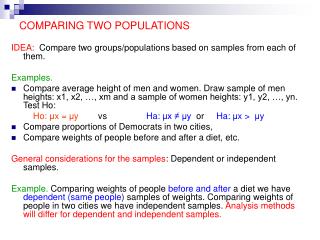
Inference for the difference of two parameters • Often we are interested in comparing the population average or the population proportion/percentage for two groups • We can do these types of comparisons using CI’s and hypothesis tests • General ideas and equations don’t change • CI: estimate ± multiplier*SE • Test statistics: (observed– expected)/SE
Inference for P1 – P2 • Lets just jump right into an example
CI for P1 – P2 • Estimate ± multiplier*SE • Multiplier comes from the z-table • Everything else we know about confidence intervals is the same • Interpretation • What does 95% confidence mean
Inference for difference of two population means μ1 – μ2 • Two possibilities in collecting data on two variables here • Design 1: Units are matched in pairs • Use “matched pairs inference” • Design 2: units not matched in pairs • Use “two sample inferences”
Typical study designs • Matched pairs • A) two treatments given to each unit • B) units paired before treatments are assigned, then treatments are assigned randomly within pairs • Two samples • A) some units assigned to get only treatment a, and other units assigned to get only treatment b. Assignment is completely at random • B) Units in two different groups compared on some survey variable
Matched pairs vs two samples • Data collected in two independent samples: • No matching, so creating values of some “difference” is meaningless • A “matched pairs” analysis is mathematically wrong and gives incorrect CI’s and p-values • Data collected in matched pairs: • Matching, when effective, reduces the SE. • A two sample analysis artificially inflates the SE, resulting in excessively wide CI’s and unreliable p-values • An example towards the end of these slides will demonstrate this
Inference in μ1 – μ2: matched pairs • General idea with matched pairs design is to compute the difference for pair of observations and treat the differences as the single variable • Measure y1 and y2 on each unit. Then for each unit compute • d = y1 – y2 • Then find a confidence interval for the difference • difference estimate ± multiplier*SE • average of differences ± t-table value * SD of differences/√n
Inference in μ1 – μ2: matched pairs • Do people perform better on tests when smelling flowers versus smelling nothing? • Hirsch and Johnston (1996) asked 21 subjects to work a maze while wearing a mask. The mask was either unscented or carried a floral scent. Each subject worked both mazes. The order of the mask was randomized to ensure fair comparison to the two treatments. The response is the difference in completion times for the unscented and scented masks. • Example: Person 1 completed the maze in 30.60 seconds while wearing the unscented mask, and in 37.97 seconds while wearing the scented mask. • So, this person’s data value is –7.37 (30.60 – 37.97).
JMP output for odor example • The differences appear to follow the normal curve. There are no outliers • Sample average difference is 0.96, suggesting people do better with scented mask
Conclusions from odors example • The 95% CI ranges from -4.76 to 6.67, which is too wide a range to determine whether floral odors help or hurt performance for these mazes. In other words, the data suggest that any effect of scented masks is small enough that we cannot estimate it with reasonable accuracy using these 21 subjects. We should collect more data to estimate the effect of the odor more precisely. • We also note that this study was very specific. The results may not be easily generalized to other populations, other tests, or other treatments.
Inference in μ1 – μ2: two samples • Pygmalion study • Researchers gave IQ test to elementary school kids. • They randomly picked six kids and told teachers the test predicts these kids have high potential for accelerated growth. • They randomly picked different six kids and told teachers the test predicts these kids have no potential for growth. • At end of school year, they gave IQ test again to all students. • They recorded the change in IQ scores of each student. • Let’s see what they found…
EDA for pygmalion study • It looks like being labeled “accelerated” leads to larger improvements than being labeled “no growth” • Let’s make a 99% CI to confirm this
Sample means and SD’s Level Number Mean SD SE accelerated 6 15.17 4.708 1.92 none 6 6.17 3.656 1.49 Sample difference is 9.00. The SE of this difference:
Pygmalion confidence interval • 99% CI for difference in mean scores (accel – none): • Estimate ± mulitplier*SE • Estimate is mean1 – mean2 • Multiplier comes from the t-table (we will talk about df in a sec.) • SE of difference from the previous slide
Conclusions from the pygmalion study • The 99% CI ranges from 1.30 to 16.70, which is always positive. The data provide evidence that students labeled “accelerated” have higher avg. improvements in IQ than students labeled “no growth.” We are 99% confidence the difference in averages is between 1.3 and 16.7 IQ points.
Degrees of Freedom • Use the Welch-Satterhwaite degrees of freedom formula • This is typically what a computer will give you • Conservative approach use the smaller of n1-1 and n2-1
Hypothesis tests for difference of two parameters • The main ideas of hypothesis tests remain the same • 1) specify hypothesis • 2) compute test statistic (observed – expected)/SE • 3) calculate p-value • 4) make conclusions
Hypothesis test for p1 – p2 • Herson (1971) examined whether men or women are more likely to suffer from nightmares. He asked a random sample of 160 men and 192 women whether they experienced nightmares “often” (at least once a month) or “seldom” less than once a month • In the sample 55 men (34.4%) and 60 women(31.3%) said they suffered nightmares often. Is this 3.1% difference sufficient evidence of a sex-related difference in nightmare suffering?
Hypothesis test for p1 – p2 • Step 1: Claim is mean and women suffer at different raties • Ho: p1 = p2 vs Ha p1 ≠ p2 the same as • Ho: p1 – p2 = 0 vs Ha p1 – p2 ≠ 0 • Step2: Compute test statistic
Hypothesis test for p1 – p2 • Step 2 continued • Notice that the test statistic is simply the # of SE’s the sample difference in proportions is from 0 (the hypothesized difference). • Step3: Compute the p-value • Since we are dealing with a two-sided alternative we want the area under the normal curve to left of -0.62 and to the right 0f 0.62 • P-value ≈ 0.55
Hypothesis test for p1 – p2 • Step 4 make a conclusion • This is a large p-value. We do not reject the null hypothesis. The data do no provide sufficient evidence to concluce that the proportion of men that have nightmares is different from that of women. • As a reminder how do we interpret the value 0.55 • Assuming the null hypothesis is true (i.e. men and women are equally likely to have nightmares), there is a 55% chance of getting a sample difference of 3.1% or more (in either direction)
Inference in μ1 – μ2: matched pairs • Do people perform better on tests when smelling flowers versus smelling nothing? • Hirsch and Johnston (1996) asked 21 subjects to work a maze while wearing a mask. The mask was either unscented or carried a floral scent. Each subject worked both mazes. The order of the mask was randomized to ensure fair comparison to the two treatments. The response is the difference in completion times for the unscented and scented masks. • Example: Person 1 completed the maze in 30.60 seconds while wearing the unscented mask, and in 37.97 seconds while wearing the scented mask. So, this person’s data value is –7.37 (30.60 – 37.97).
JMP output for odor example • The differences appear to follow the normal curve. There are no outliers. • The sample average difference is 0.96, suggesting people do better with the scented mask
Hypothesis test for μ1 – μ2: matched pairs • Claim: smelling flowers helps you complete maze faster • Ho: μf = μh vs. Ha:μf < μh • Ho: μf - μh = 0vs. Ha:μf - μh < 0 • Ho: D= 0vs. Ha: D< 0 • Test statistic
Conclusions about odor • Using a t-distribution with 20 (21 – 1) degrees of freedom, the p-value is Pr(T<-0.349) = 0.3652.Assuming there is no difference in average scores when wearing either mask, there is a 36.52% chance of getting a sample mean difference of .957 seconds favoring the scented mask. This is a non-trivial chance. Therefore, we do not have enough evidence to conclude that wearing a scented mask improves performance on the maze.
Inference in μ1 – μ2: Two independent samples • Pygmalion study revisited (starts on slide 14) • Step1 Ho: μa = μn vs. Ha:μa > μn • Step2 • Step3 find the p-value. We use the t-table with how many degrees of freedom? Use 10 as in the CI • p-value between smaller than 0.01 • We will reject Ho. • Strong evidence in data to conclude that those labeled “accelerated” have larger IQ scores than those being labeled “no growth”
Matched pairs analysis • MPG for 10 cars collected after similar drives using each of two different types of gas additiv • Matched pairs analysis Variable N mean SD SE diff(a – b) 10 -0.82 0.61 0.19 • 95% CI for mean difference (-1.256, -0.384) • P-value = 0.002 • Two sample analysis Variable N Mean SD SE Mpg a 10 20.6 14.1 4.4 Mpg b 10 21.4 14.2 4.4 • 95% CI for difference (-14.14, 12.50) • P-value = 0.898
Conclusions from previous example • Right analysis (matched pairs) has narrow CI and tiny p-value. We are able to see that additive b yields more miles per gallon. • Wrong analysis (two independent samples has a very wide CI and a large p-value. Using this analysis we’d incorrectly conclude additives a and b are equally effective • Here’s why • Variation in mpg across cars is much higher than variation in mpg within cars. By matching we eliminate this across-car variation. The two-independent samples analysis ignores elimination of across-car variance • Moral of the story: Use anlaysis that corresponds to how data are collected
Matched pairs cont. • Why not always use matched pairs? • Matching increases the possibility of imbalance in background variables. Matching on irrelevant variables can make inferences less precise because of imbalance in causally-relevant background variables. • Guidance for using matched pairs? • Match on variables that have substantial effect on response. This can make inferences more precise.
Determining a sample size • We will use a method that is sometimes called the “margin of error method” • Suppose we want a 95% CI for the percentage of people who show symptoms of clinical despression • Further more we want the CI to be fairly precise: we want a margin of error of 1% • Therefore we want
Determining sample size • Using we can solve for n • Now you just plug in your best guess for P and you have the sample size required for a 1% margin of error • Ex: say that P=0.3 • If this sample size is too expensive either decrease level of confidence or desired maring of error
Determine sample size for differences in % and average • Same logic applies • Write down the expression for SE • Decide on a margin of error • Solve for sample size • Guess P1 and P2 for differences in two percentages and SD1 and SD2 for differences in means • Set n1 = n2 (same sample size for each group)
Determining sample size • The same ideas apply with you desire a CI of a mean • Suppose that we want to estimate the average weight of men in the U.S. • Further suppose that we want a margin of error to be 8 pounds • We need to guess at the SD for weight. Let’s guess it to be around 20 punds • Then solving for n we get • Round up and take a sample of 25
Determining sample sizes for differences in % and avg. • Same logic applies: • Write down expression of SE • Decide on a desired margin of error • Solve for sample size • Guess p1 and p2 for difference in two percentages. • Guess SD1 and SD2 for differences in two means. • Set n1 = n2 . Sample size in each group is n1