Download
1 / 31
320 likes | 574 Views
Vision Review: Image Formation. Course web page: www.cis.udel.edu/~cer/arv. September 10, 2002. Announcements. Lecture on Thursday will be about Matlab; next Tuesday will be “Image Processing”

E N D
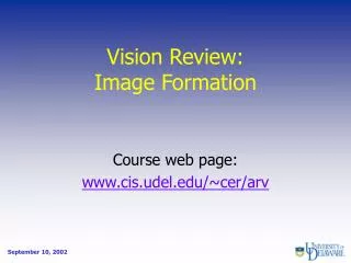
Vision Review:Image Formation Course web page: www.cis.udel.edu/~cer/arv September 10, 2002
Announcements • Lecture on Thursday will be about Matlab; next Tuesday will be “Image Processing” • The dates some early papers will be presented are posted. Who’s doing what is not, yet (except that I’m the first two). • In particular, read “Video Mosaics” paper up to “Projective Depth Recovery” section • Supporting readings: Chapters 1, 3 (through 3.3.2 “Hue, Saturation, and Value” subsection), 5 (through 5.3.2), and 7.4 of Forsyth & Ponce
Computer Vision Review Outline • Image formation • Image processing • Motion & Estimation • Classification
Outline: Image Formation • Geometry • Coordinate systems, transformations • Perspective projection • Lenses • Radiometry • Light emission, interaction with surfaces • Analog Digital • Spatial sampling • Dynamic range • Temporal integration
Coordinate System Conventions • unit vectors along positive axes, respectively; • Right- vs. left-handed coordinates • Local coordinate systems: camera, world, etc.
Homogeneous Coordinates (Projective Space) • Let be a point in Euclidean space • Change to homogeneous coordinates: • Defined up to scale: • Can go back to non-homogeneous representation as follows:
3-D Transformations:Translation • Ordinarily, a translation between points is expressed as a vector addition • Homogeneous coordinates allow it to be written as a matrix multiplication:
3-D Rotations: Euler Angles • Can decompose rotation of about arbi-trary 3-D axis into rotations about the coordinate axes (“yaw-roll-pitch”) • , where: (Clockwise when looking toward the origin)
3-D Transformations:Rotation • A rotation of a point about an arbitrary axis normally expressed as a multiplication by the rotation matrix is written with homogeneous coordinates as follows:
3-D Transformations: Change of Coordinates • Any rigid transformation can be written as a combined rotation and translation:
3-D Transformations: Change of Coordinates • Points in one coordinate sytem are transformed to the other as follows: • (taking the camera to the world origin) represents the camera’s extrinsic parameters
Pinhole Camera Model Image plane Optical axis Principal point Focal length Camera center Camera point Image point
Pinhole Perspective Projection • Letting the camera coordinates of the projected point be leads by similar triangles to:
Projection Matrix • Using homogeneous coordinates, we can describe perspective projection with a linear equation: (by the rule for converting between homogeneous and regular coordinates)
Camera Calibration Matrix • More general projection matrix allows: • Image coordinates with an offset origin (e.g., convention of upper left corner) • Non-square pixels • Skewed coordinate axes • These five variables are known as the camera’s intrinsic parameters
Combining Intrinsic & Extrinsic Parameters • The transformation performed by a pinhole camera on an arbitrary point can thus be written as: • is called the camera matrix
Homographies • 2-D to 2-D projective transformation mapping points from plane to plane (e.g., image of a plane) • 3 x 3 homogeneous matrix defines homo-graphy such that for any pair of corresponding points and , from Hartley & Zisserman
Computing the Homography • 8 degrees of freedom in , so 4 pairs of 2-D points are sufficient to determine it • Other combinations of points and lines also work • 3 collinear points in either image are a degenerate configuration preventing a unique solution • Direct Linear Transformation (DLT) algorithm: Least-squares method for estimating
DLT Homography Estimation:Each of n Correspondences • Since vectors are homogeneous, are parallel, so • Let be row j of , be stacked ‘s • Expanding and rearranging cross product above, we obtain , where
DLT Homography Estimation:Solve System • Only 2 linearly independent equations in each , so leave out 3rd to make it 2 x 9 • Stack every to get 2n x 9 • Solve by computing singular value decomposition (SVD) ; is last column of • Solution is improved by normalizing image coordinates before applying DLT
Applying Homographies to Remove Perspective Distortion from Hartley & Zisserman 4 point correspondences suffice for the planar building facade
Homographies for Bird’s-eye Views from Hartley & Zisserman
Homographies for Mosaicing from Hartley & Zisserman
Camera Calibration • For a given camera, how to deduce so we’ll be able to predict the image locations of known points in the world accurately? • Basic idea: take images of measured 3-D objects, estimate camera parameters that minimize difference between observations and predictions
Estimating K • Now we have a 3-D to 2-D projective transformation described by • Follow approach of DLT used for homography estimation, except now: • is 3 x 4, so need 5 1/2 point correspondences • Degeneracy occurs when 3-D points are coplanar or on a twisted cubic (space curve) with camera • Use RQ decomposition to separate estimated into and
Real Pinhole Cameras • Actual pinhole cameras place the camera center between the image plane and the scene, reversing the image • Problem: Size of hole leads to sharpness vs. dimness trade-off • A really small hole introduces diffraction effects • Solution: Light-gathering lens A (fuzzy) pinhole image courtesy of Paul Debevec
Lenses • Benefits: Increase light-gathering power by focusing bundles of rays from scene points onto image points • Complications • Limited depth of field • Radial, tangential distortion: Straight lines curved • Vignetting: Image darker at edges • Chromatic aberration: Focal length function of wavelength
Correcting Radial Distortion courtesy of Shawn Becker Distorted After correction
Modeling Radial Distortion • Function of distance to camera center • Approximate with polynomial • Necessitates nonlinear camera calibration
Camera Calibration Software • Examples of camera calibration software in Links section of course web page • Will discuss Bouguet’s Matlab toolbox on Thursday courtesy of Jean-Yves Bouguet