Download
1 / 43
460 likes | 683 Views
Learn about whole-genome optical mapping technology for studying human genome variation, including substitutions, duplications, and rearrangements. Understand the process of optical mapping, data analysis, errors, and pros and cons. Discover the goals of optical mapping, map-making approaches, and assembly techniques using overlap-layout-consensus paradigm. Explore the challenges and solutions in optical map assembly and overlap detection.

E N D
Whole-Genome Optical Mapping Michael Waterman University of Southern California
Human Genome Variation • Types of Variation Substitutions Insertion/deletions Duplications Rearrangements SNPs: single nucleotide polymorphisms
Optical Mapping • A single-molecular restriction mapping technology • Developed by D. Schwartz (University of Wisconsin-Madison)
Optical Mapping: Overview + DNA extract Molecules attached to the surface and straightened within the grooves Silicon bed with embedded grooves Restriction enzymes are added in the solution DNA is fluorescently dyed and the chip is photographed. DNA is digested and cuts are formed by shrinking ends
DNA Imaging Lambda DNA individual fragments cuts Estimated sizes of fragments
Optical Mapping: Data • Each optical map is represented by an array of DNA sizes in the order they appear on imaged DNA molecules. • Individual maps correspond to different DNA molecules of length 0.3-1.5 Mb. • Each number in the map corresponds to size of the restriction fragment (in Kb) on the molecule. • Order information of restriction fragments is preserved within each map. Map #1: 10.23 54.32 32.43 12.43 9.54 0.45 3.98 2.76 3.45 19.23 27.81 92.12 0.65 4.22 Map #2: 23.12 68.42 28.12 15.43 12.92 32.90 0.34 0.78 5.43 54.22 29.69 27.12 14.23 13.08 0.54 12.35 22.19 1.34 ...
Optical Mapping: Errors • Sizing errors (sizes of individual restriction fragments are measured with errors) • Missing cuts (due to underdigestion) • False cuts (random DNA breaks) • Missing fragments (unable to attach to the surface) • Chimeras (due to concatenation of maps during imaging)
Optical Mapping: Pros and Cons • Pros: • No cloning, no amplification, hence no PCR related errors. • Deep (~100x and more) coverage • Reads span very large portions of chromosomes ~(up to 4Mb). • Cons: • Resolution at the restriction site level • Maps contain many errors
Optical Mapping: Goals • Assembly of restriction maps for target organisms (before sequencing) • Variation studies (cancer analysis) • Mapping of methylation patterns • Mapping of transcription factor binding sites
Map Making • We are confronted with many relatively short somewhat inaccurate maps and want to piece together a genome map • The problem was approached by a sophisticated statistical sampling model by Mishra et al. • We try another quite simple approach
Overview: Assembly for Sequences (Overlap – Layout – Consensus Paradigm) Genomic region cloning, sequencing Overlap GTTGA Physical overlaps between reads are captured by means of filtration Piles of sequence reads (~600Bp each) GTTGA ATGATCC Filtration ATGATCC Overlapping sequence reads are put together to produce the scaffold of the reference genomic region (Layout) Layout Consensus map is inferred by means of multiple sequence alignment, Euler assembler, etc. Consensus
Assembly for Optical Maps: Overlap-Layout-Consensus • Overlaps are computed according to our new probabilistic score • Layout is produced similar to sequence layout • Consensus is inferred by refinement of the layout (HMM) Mutual overlaps are detected by finding similar size patterns Overlap Filtration significantly speeds up the computation of overlaps Filtration
Assembly for Optical Maps: Overlap Detection • Huge number of false positive overlaps • False negatives (missing overlaps) are not a problem for layout construction • Many optical maps, hence all pairwise overlaps are expensive to calculate ( n(n-1) overlaps, if n optical maps ) • Filtration is needed to speed up the search for overlaps
Assembly for Optical Maps: Filtration • Filtration is used to find: • Potential overlaps of optical maps • Possible fit locations against the reference • Filtration is based on finding matching tuples of fragments for optical maps: • Matching tuples are calculated to form matching diagonal stretches in the alignment matrix • Matching diagonal stretches in the alignment matrix are chained to find alignments and calculate the score (FASTA idea) • Full dynamic programming is applied for candidate overlaps to calculate the overlap
Filtration continued • In sequences overlapping reads are expected to have several matching 20-tuples • In Optical Mapping filtration is challenging because of the sizing error and presence of missing/false cuts
Assembly for Optical Maps: Why Things are Hard • Consider a human size genome (3 000 K bp) • Av. rf size 30K (8-cutter), hence 100K restriction fragments in 1 genome • With maps of 33 rf (1 Mbp) there is • 1x – 3K maps • 100x – 300K maps • pair-wise overlaps • To calculate all pair-wise overlaps: • At the rate of 5 overlaps per second or overlaps per hour • computer hours • 4.5 years on the 128 node cluster like hto-g.
Alignment Score: Problem Description • Account for features specific for optical mapping: • Sizing error distribution • False cut distribution • Missing cut distribution • Design a score as a –log(LR) for testing: true matching vs. random matching: • True match assumes direct dependence between maps • Random match assumes independence between maps • The optimal alignment has the lowest LR-test value (maximum score)
Previous work on the subject • Heuristic alignment score and DP for restriction map alignments (Waterman et al, 1984) • Alignment score and DP for restriction maps with local rearrangements (Huang et al, 1992) • Extensive Bayesian models for map assemblies (Ananthraman et al, 1997)
Optical Mapping: Calculation of Alignments • Alignments are computed using standard DP algorithm for map comparison (due to Waterman et al, 1984) • Time complexity: , but can be approximated by a restricted version is the size of the reference map is the size of the optical map
Optical Mapping: Data Models • Sizing errors (about 10-15% of the fragment size) • Modeled as normal r.v. • for fragments longer than 4 Kb (CLT idea) • for fragments shorter than 4 Kb • About 20% of cuts are missing (80% digestion) • Modeled as Bernoulli r.v. • False cuts occur at the rate of 5 per Mb • Modeled as Poisson Process with rate 0.005
Why normal error model? Fluorescent dye • Let be the # of photons captured from the i-th base • The total registered fluorescence from the DNA fragment is (n DNA bases) • After applying CLT for an unbiased measurement , since L is proportional to n • Hence for the measurement error DNA
Testing the Error model: Scatter Plot vs Histogram of Data collected from 10-mers.
Error model: qqnorm Data collected from 10-mers.
Alignment Score: Key Idea • Define two competing hypothesis and : • under maps and are independent (have no similarity) • under maps and are related (e.g. optical map comes from the genomic region ) • write the likelihood ratio under and :
Alignment Score: Key Idea • define an alignment score as the –log(LR) to make it additive:
Two Alignment Types: Fit and Overlap • Fit alignment: to find genomic regions of origin for optical maps Sizing errors Reference restriction map Aligned pairs of sites Missed cut False cut • Overlap alignment: to detect overlaps between optical maps Aligned pairs of sites Optical maps
Optical Mapping: Alignment Scores Matching regions • Score of the matching region is composed of two parts: score for the sizing error and score for extra/missing cut sites R R R 2 d Score = score(R ) + score(R ) + . . . + score(R ) 1 2 d
Comparison of two alignment scores • M1: Our alignment score • M2: Alignment score due to Waterman et al 1984 • P-values are consistently smaller for our new score
Comparison of two alignment scores • Generate a map from a 40 MB region of HS13. • Verify that optimal score places into a correct genomic location • Examine 19 next best scoring alignments • Study how sparsely populated are the neighborhoods of optimal alignments using M1 and M2 (using std of optimal score) • For our new score (M1): neighborhoods of optimal scores are very sparsely occupied • For the old score (M2): neighborhoods of optimal score are densely occupied
Tumor study: analysis of variations • Variations to find: • indels (5Kb or more) • extra or missing restriction cut sites (EC or MC) • Variations are relative to published DNA human sequence (build 35) • Data: • human hematadiform mole (haploid, @12x) • limphoblastoid control (diploid white blood cells, @8x)
Selected variations • By p-value (<0.05) • Discovered: • Lymphoblastoid (normal white blood cell), 8x, 63% cov: • 131 indel (>5Kb) • 491 EC • 609 MC • Mole (Haploid tumor), 12x, 93% cov: • 728 indels (>5Kb) • 394 EC • 489 MC
Mole: indels 501 out of 728 indels are 5-10 Kb deletions
Why such a difference? • Hypothesis: L1 line elements: • 6-8Kb retrotransposons: • Pop out in mole • Stay in place in normal cells • Hypothesis: EC, MC are due to SNPs at the restriction sites
Our Research Group: • Michael Waterman (USC) • Lei Li (USC) • Yi Yang (USC) • Yu-Chi Liu (USC) • Yu Zhang (Harvard) • Anton Valouev (USC) & Many many thanks to David Schwartz and his Lab (U.Wisconsin)