Data Assimilation: Combining Measurements and Models for Environmental System Characterization

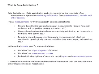
1. What is Data Assimilation ? • Data Assimilation: Data assimilation seeks to characterize the true state of an environmental system by combining information from measurements, models, and other sources. • Typical measurements for hydrologic/earth science applications: • Ground-based hydrologic and geological measurements (stream flow, soil moisture, soil properties, canopy properties, etc.) • Ground-based meteorological measurements (precipitation, air temperature, humidity, wind speed, etc.) • Remotely-sensed measurements (usually electromagnetic) which are sensitive to hydrologically relevant variables (e.g. water vapor, soil moisture, etc.) • Mathematical models used for data assimilation: • Models of the physical system of interest. • Models of the measurement process. • Probabilistic descriptions of uncertain model inputs and measurement errors. A description based on combined information should be better than one obtained from either measurements or model alone.

2. Key Features of Environmental Data Assimilation Problems State estimation -- System is described in terms of state variables, which are characterized from available information Multiple data sources -- Estimates are often derived from different types of measurements (ground-based, remote sensing, etc.) measured at different times and resolutions. State variables may fluctuate over a wide range of time and space scales -- Different scales may interact (e.g. small scale variability can have large-scale consequences) Spatially distributed dynamic systems -- Systems are often modeled with partial differential equations, usually nonlinear. Uncertainty -- The models used in data assimilation applications are inevitably imperfect approximations to reality, model inputs may be uncertain, and measurement errors may be important. All of these sources of uncertainty need to be considered in the data assimilation process. The equations used to describe the system of interest are usually discretized over time and space -- Since discretization must capture a wide range of scales the resulting number of degrees of freedom (unknowns) can be very large.

3. State-Space Framework for Data Assimilation • State-space concepts provide a convenient way to formulate data assimilation problems. Key idea is to describe system of interest in terms of following variables: • Input variables -- variables which account for forcing from outside the system or system properties which do not depend on the system state. • State variables -- dependent variables of differential equations used to describe the physical system of interest, also called prognostic variables. • Output variables -- variables that are observed, depend on state and input variables, also called diagnostic variables. Classification of variables depends on system boundaries: Atmosphere Atmosphere Precip. ET Precip. ET Land Land System includes coupled land and atmosphere -- precipitation and evapo-transpiration are state variables System includes only land, precipitation and evapo-transpiration are input variables

4. Time-varying input u(t) (e.g. precip) State y (t) (e.g. soil moist.) Hydrologic system Measurement system Specified (mean) True True True Random fluctuations Output zi (e.g. radiobrightness) Random error,  Random fluctuations Specified (mean) Measured Time-invariant input  (e.g. sat. hydr. cond.) Data assimilation algorithm Means and covariances of true inputs and output measurement errors Estimated states and outputs State Eq: Measurement Eq: Components of a Typical Hydrologic Data Assimilation Problem The data assimilation algorithm uses specified information about input fluctuations and measurement errors to combine model predictions and measurements. Resulting estimates are extensive in time and space and make best use of available information.

5. Types of Measurement Errors • When models are discretized over time/space there are two sources of output measurement error: • Instrument errors (measurement device does not perfectly record variable it is meant to measure). • Scale-related errors (variable measured by device is not at the same time/space scale as corresponding model variable) 3.5 4 * * Large-scale trend described by model 3 3 Instrument error 2 2.5 * 1 True value 2 * Scale-related error 0 1.5 Measurement -1 1 -2 100 101 102 90 95 100 105 110 115 120 When measurement error statistics are specified both error sources should be considered

6. Types of Data Assimilation Problems - Temporal Aspects Interpolation: no time-dependence, characterize system only at time t=ti Use for interpolation of spatial data (e.g. kriging) t1 t2 t ti Smoothing: characterize system over time interval t ti Use for reanalysis of historic data t=ti Filtering/forecasting: characterize system over time interval t ti Use for real-time forecasting t t1 t2 ti Zi = [z1, z2, …, zi] =Set of all measurements through time ti

7. Types of Data Assimilation Problems - Spatial Aspects Downscaling: Characterize system at scales smaller than output measurement resolution Upscaling: Characterize systemat scales larger than output measurement resolution Measurement (z1 ) States (y1 … y4) Measurements (z1 ...z4) State (y1) Downscaling and upscaling are handled automatically if measurement equation is defined approriately

8. u: p(u) p(u | Zi) p[y(t)| Zi] y = A(u) Std. Dev. y: p(y) p(y | Zi) Prior Conditional Zi Mode Mean y(t) Characterizing Uncertain Systems What is a “good characterization” of the system states and inputs, given the vector Zi = [z1, ..., zi] of all measurements taken through ti? The posterior probability densitiesp(y| Zi) and p(u| Zi) are the ideal estimates since they contain everything we know about the state y or input u given Zi. In practice, we must settle for partial information about this density • Variational DA: Derive mode of p[y(t)| Zi] by solving batch least-squares problem. • Sequential DA: Derive recursive approximation of conditional mean (and covariance?) of p[y(t)| Zi]

9. Most variational methods use the mode of p u|z(u| Zi) as an estimate of uncertain input vector. State estimate is obtained by substituting into state equation: If  and u are multivariate normal is the value of that minimizes the following generalized least-squares error measure: Terms that do not depend on u2 is found with an iterative search. Search convergence is improved by the presence of the second (regularization) term in JB. u1 The Variational/Batch Approach The state equation is often incorporated as a constraint, using adjoint methods.

10. The Sequential Approach Meas. i Meas. 1 Meas. 2 zi z1 z2 Zi= [Zi-1 , zi] Z1= [z1] Z2= [Z1 , z2] t0 t1 t2 ti ti+1 p y2| z1[ y2|Z1 ] p y1[ y1] p yi| zi-1[ yi|Zi-1] p y,i+1| zi[ yi+1|Zi ] Propagation i to i+1 Propagation 0 to 1 Propagation 1 to 2 p y0[ y0] p y1| z1[ y1|Z1 ] p yi| zi[ yi|Zi ] Algorithm initialized with unconditional (prior) PDF at t0 Update 1 Update i Sequential methods are designed to propagate and update the conditional pdf in a series of discrete steps: In practice various approximations must be introduced.

11. Some Common Sequential Data Assimilation Methods Propagated estimate update A common approximation is to assume that the conditional PDF is multivariate Gaussian. The update for conditional mean has the form: K weights measurements vs. model predictions Some common approximations: Direct Update forced to equal measurements where available, insertion interpolated from meas. elsewhere Nudging: K = empirically selected constant Optimal K derived from assumed (static) covariance Interpolation: Extended K derived from covariances propagated with a linearized Kalman filter: model, input fluctuations and measurement errors must be additive. Ensemble K derived from a ensemble of random replicates propagated Kalman filter: with a nonlinear model, form of input fluctuations and measurement errors is unrestricted.

12. 1 sand silt 0.9 clay 0.8 microwave emissivity [-] 0.7 0.6 0.5 0 0.2 0.4 0.6 0.8 1 saturation [-] Example -- Microwave Measurement of Soil Moisture L-band (1.4 GHz) microwave emissivity is sensitive to soil saturation in upper 5 cm. Brightness temperature decreases for wetter soils. Objective is to map soil moisture in real time by combining microwave meas. and other data with model predictions (data assimilation).

13. Case Study Area Aircraft microwave measurements SGP97 Experiment - Soil Moisture Campaign

14. Problem Specifications –SGP97 Ensemble Kalman Filter Example • Hydrologic model: 1D (vertical) NOAH Land Surface Model (NOAA NCEP, Chen et al, 1996) applied at each estimation pixel • Radiative Transfer Model: Jackson et al , 1999 model applied at each pixel • Uncertain model inputs included in ensemble filter: Time-varying inputs: Precipitation (temporally uncorrelated) Time-invariant inputs: Porosity (upper bound on moisture content) Wilting point (lower bound on moisture content) Saturated hydraulic conductivity Minimum stomatal resistance Random fluctuations are multiplicative and lognormal (mean=1.0) • Random measurement errors included in ensemble filter: • Additive radiobrightness measurement noise • Filter assumes that random fluctuations and measurement errors for different pixels are uncorrelated

15. Relevant Time and Space Scales 0.025 0.02 * * * * * * * * * * * * * * * 0.015 mm/s 0.01 0.005 0 170 175 180 185 190 195 5 cm 10 cm Typical precipitation events Plan View Estimation pixels (large) Microwave pixels (small) * = ESTAR observation 0.8 km 0.8 km 4.0 km 170 = 6/19/97 Vertical Section Soil layers differ in thickness Note large horizontal-to-vertical scale disparity For problems of continental scale we have ~ 105 est. pixels, 105 meas, 106 states,

16. Some Typical Spatially Variable Model Inputs –SGP97 Example Sand fraction 50 km 0 0.2 0.4 0.6 0.8 NOAH soil class NOAH vegetation class Meteor. Stations RTM Inputs Clay fraction El Reno 0 2 4 6 8 0 2 4 6 8 10 12 NOAH Inputs 0 0.05 0.1 Estimation region ~ 50 by 200 km (12 by 50 pixels 4 km on a side)

17. Brightness Temperatures at a Typical Pixel – SGP97 Example Brightness meas. Individual replicates Conditional mean Unconditional mean Precip Brightness Temp. and Precip Time Series – El Reno Brightness temp. deg. K.

18. Moisture Contents at a Typical Pixel – SGP97 Example Brightness meas. times Individual replicates Conditional mean Unconditional mean Local spatial average of gravitimetric meas. Precip Moisture Content and Precip. Time Series – El Reno Moisture content

19. Comparison of Some Data Assimilation Options Direct insertion, nudging, optimal interpolation Variational methods • Easy to implement + • Updates do not account for system dynamics or input and measurement statistics – • No information on estimation accuracy – • Computationally efficient + • Well-suited for smoothing problems, less convenient for real-time applications +/- • Does not provide information on estimation accuracy - • Difficult to accommodate time-dependent model errors, not robust – • Most efficient forms require derivation of an adjoint model - Extended Kalman filter • Can be adapted for real time or smoothing problems + • Provides info. on estimation accuracy + • Computationally demanding, limited capability to deal with model errors - • Linearization approximation may be poor, tends to be unstable - Ensemble Kalman filter • Well-suited for real time applications, not optimal for smoothing problems +/- • Provides information on estimation accuracy + • Very flexible, modular, able to accommodate wide range of model error descriptions + • No need for adjoint model or for linearizations or other approximations during propagation step + • Approach is robust and easy to use + • Update assumes states are jointly normal– • Can be computationally demanding–