Auction Algorithms for Market Equilibrium
280 likes | 368 Views
Auction Algorithms for Market Equilibrium. Rahul Garg IBM India Research Sanjiv Kapoor Illionis Institute of Technology. Overview. The market equilibrium problem History and recent developments A parameterized linear programming formulation The auction algorithm

Auction Algorithms for Market Equilibrium
E N D
Presentation Transcript
Auction Algorithms for Market Equilibrium Rahul Garg IBM India Research Sanjiv Kapoor Illionis Institute of Technology
Overview • The market equilibrium problem • History and recent developments • A parameterized linear programming formulation • The auction algorithm • Analysis and proof outline • Conclusions and future work
A (Fisher) Market • There are n buyers and m sellers • Each seller has exactly one commodity(seller j has aj amount of commodity j) • Buyers have only money(buyer i has ei units of money) • Sellers want only money, buyers want only commodities
A (Fisher) Market • Buyers have utilities on commodity bundlesui: R+m R+The utility function ui of buyer i maps an endowment of commodities to a “happiness” index • The buyers and sellers come to the market and exchange commodities to maximize happiness • Each buyer and seller acts independently to maximize its own happiness
The General Market Model (Walras) • There are n traders and m commodities • Each trader has initial endowments of commodities aij = amount of commodity j with trader i • Traders have utilities on commodity bundlesui: R+m R+The utility function ui of trader i maps an endowment of commodities to a “happiness” index • The traders come to the market and exchange commodities to maximize happiness • Each trader acts independently and acts to maximize its own happiness
Market Equilibrium • Commodities are divisible • xij: the amount of commodity j with trader i after the trade • Commodity j is tagged with a price pj • xij is a solution to the optimization problem • No excess or deficiency of any commodity
Market Equilibrium • No incentive for a trade • No deficiency or surplus of any commodity • p1, p2, …, pm are equilibrium prices • Prices are in terms of an abstract currency • Prices invariant to scaling • Real money is a commodity (say m) • Real price of commodity j is pj / pm • Not an optimization problem
Market Equilibrium History • Posed by • 1891 Fisher • 1894 Walras (Walrasian Equilibrium) • Existence • 1954 Arrow and Debreu • Computation • Hydraulic apparatus by Fisher • Walrasian tatonnement • Convergence? • Polynomial time algorithms?
Computation of Market Equilibrium • Arrow et al. 1959 • Stability of a local greedy price adjustment method for “Gross Substitute” utility functions • Eisenberg and Gale, 1959 • Fisher model, additive linear utilities • Optimization problem • Eaves, 1976 • Linear complementarity problem • Lemke’s algorithm • Newman and Primak, 1992 • Ellipsoid method – provably polynomial-time method
Computation of Market Equilibrium • Devanur et al. 2002 • Fisher model, separable additive and linear utilities • Combinatorial algorithm based on max flows • Complexity: n4/ max-flow computations ~ n7/ • Jain et al 2003, Devanur and Vazirani 2003 • Approximation algorithm for Walrasian model, linear utilities • Jain, 2004 • General Walrasian model, additive linear utilities • Ellipsoid method (similar to Eisenberg and Gale) • Ye 2004 • Fisher and Walrasian model, linear utilities • Complexity: n4 L
Algorithms for Market Equilibrium • Centralized • Slow • Very difficult to define and report utility functions • Impractical
Auction Algorithms for Market Equilibrium • Fisher and General Walrasian model • Additive linear utilities • Approximation algorithm • Decentralized and distributed • Very simple • Natural auction interpretation • Complexity: 1/ (n m2 + m n2) log vmax steps
The Market Equilibrium Problem • Linear, additive utilities
A Parameterized LP Formulation • A family of LPs • pj are market clearing prices iff there is a dual optimal with = 0 Search for p such that optimal dual has = 0
The Auction Algorithm • Fix a bid increment factor (1 + ) • Start with low prices • A trader with “sufficient” surplus money finds its best commodity • a commodity that maximizes vij / pj • Acquires a best item by outbidding the current winning trader • Raises the price of the acquired commodity by (1 + ) • Stop when all the traders have small surplus
Outbidding Trader i Item j Trader k pj ykj Trader i (1 + ) pj hij yij pj Trader k (1 + ) pj hij ykj pj
Divisible Items • Every item may be sold two prices: pj and pj (1 + ) • hij amount sold at pj (1 + ) • yij amount sold at pj • Price at which item is available pj (1 + ) hij yij
Some Details • Initialize with pj = 1 for all j • Xij = hij = yij = 0 • Demand set of a trader • Di = { j: vij / pj = max vik / pk } • Surplus of a trader • ri = aij pj - yij pj - hij pj (1 + )
The Auction Algorithm while i such that ri > aij pjpick j Diif j is unassigned then get j at price 1else iff ykj > 0 for some k then outbid k on item j update ri and rk else increase pj by factor (1 + )i: yij = hij; hij = 0; recompute Di’s endifendwhile
ri rk (1 + ) pj (1 + ) pj hij hij pj yij pj yij hij yij (1 + ) pj (1 + ) pj pj hij yij pj = (1 + ) pj • ri = aij pj - yij pj • - hij(1 + ) pj • Bidding process: • Transfers surplus • Reduces it by (1 + ) • Price raise: • Increases surplus
A Primal-Dual Interpretation • Maintains dual feasibility • Satisfies complementary slackness • Successively improves primal feasibility • Stops when primal infeasibility is sufficiently small
Analysis • Terminates and achieves approximate market clearing • If order of bidding is fixed, then time complexity is good
Analysis • Number of prices raises < O(m/ log (pmax)) • Bidding in rounds • every bidders bids once in a round • either a price is raised • or r reduces by factor (1 + ) • Gives a bound of • O(1 / 2 nm log (a pmax / ( amin)) log pmax)
Aggressive Bidders • Bidder i bidding on item j • Raises prices: m / log (pmax) • Knocks out a bidder (say k) • Can a bidder get the same item again? • Yes: if j Dk • Exhausts surplus • Can surplus come again? How many times? • A modification • If i is getting j at pj then it upgrades to (1 + ) pj • If j Dk then k bids back on item immediately and gets it a price (1 + ) pj
Analysis • Define a bipartite graph G • (i, j) G iff j Di • (j, i) G iff ykj > 0 and j Di • G is acyclic • Three types of assignments • hij > 0 • yij > 0 and j Di • yij > 0 and j Di Bidders Items i j Di j k ykj > 0 and j Di
Amortization • Define Y = (j, i) : yij > 0 • Bidding • raises prices • atmost m / log (pmax) times • adds atmost n new edges in Y • exhausts an edge in Y: n m / log (pmax) times • reduces surplus to zero • atmost n2 times for every price rise • Demand set computation • atmost m / log (pmax) times • requires atmost nm steps • Requires 1/ (n m2 + m n2) log vmax) steps
Conclusions • Fast polynomial time algorithm for approximate market equilibrium – linear additive utilities • Decentralized auction algorithm • No need to reveal private information • Natural and practical • Conceivable implementation in grid economies using software agents
Future Work • Fast algorithm for exact market equilibrium (linear utilities) • Strongly polynomial time exact equilibrium algorithms • Greedy monotone price mechanisms • Separable additive gross substitute utilities • General gross substitute utilities • General (concave) utilities