Download

1 / 14
150 likes | 304 Views
Market Equilibrium. We will consider the two extreme cases Perfect Competition Monopoly. Market Equilibrium Perfect Competition. P. Supply forces (producers) and demand forces (consumers) seek a balance Price below perceived value increases demand

E N D
Market Equilibrium We will consider the two extreme cases Perfect Competition Monopoly
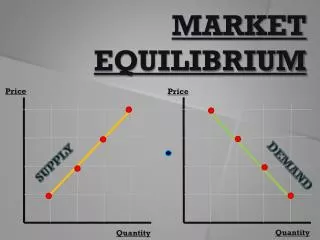
Market EquilibriumPerfect Competition P • Supply forces (producers) and demand forces (consumers) seek a balance • Price below perceived value increases demand • Price above ATC provides pure profit, an incentive to increase supply Demand curve Pe Supply curve Q
Individual Firm’s Demand and MR Curve P Highly elastic demand One firm’s change in Q has little effect on price Pe ∆P ∆Q Q
Market EquilibriumPerfect Competition • Price above ATC provides pure profit, an incentive to increase output • Pure profit equals (P1 x Q1) – (P2 x Q2) Individual Firm Price (P) MC ATC P1 P2 Q2 Q1
Market Equilibrium Perfect Competition • All firms are price takers • Market price (P1) equals marginal revenue (MR) and average revenue (AR) • Optimal level of output is where MR = MC = P1 • In long-run P will go to P2 where pure profit is eliminated Individual Firm Price (P) MC ATC P1 P2 Q2 Q1
Market Supply Curve Summation of supply curves for individual firms Q Demand Market supply curve = Qm Sum vertically Janet’s sawmill Qj + Tracy’s sawmill Qt + Pete’s sawmill Qp + Qj Joe’s sawmill P Pm (same P for all firms and market)
Perfect Competition - Example • Given supply and demand functions, Qs = 30 + 55 P Qd = 230 – 45 P • Determine marginal revenue, MR, i.e. Pe, from supply and demand curves for total market. Calculate Pe from market supply equals demand equilibrium condition, Qs = Qd 30 + 55 P = 230 – 45 P 100 P = 200 P = 2 = MR • Use P to get equilibrium quantity, Qe Qe = 230 – 45 x 2 = 230 –90 = 140
Apply Market Price to Individual Firm – “Pete’s Sawmill” P =$2 from market equilibrium Determine quantity Pete should produce from Pete’s marginal cost (MC) curve, which is, Qs = 5 + 5.8 P = 5 + 5.8 x 2 = 16.6
Market EquilibriumMonopoly • Only one producer • Producer is a price “setter”, not a price taker • Demand curve restricts ability to set price • Demand curve determines marginal revenue (MR) • Only way to change quantity sold is to change market price • Marginal revenue (MR) is not constant • What forces lead to a monopoly
Market EquilibriumMonopoly P Monopolists MC curve Pe Up & over to get P MC = MR to max. profit Market demand curve Down to get Q Monopolists MR curve Q e stands for equilibrium Qe determine fist, then get P from demand curve
Market Equilibrium Monopoly compared to competitive equilibrium P Monopolists MC curve Pm m – monopoly equilibrium c – competitive equilibrium Pc Market demand curve Monopolists MR curve Q Qm Qc
Market Equilibrium Monopoly Compared to competitive market equilibrium – Monopolist produces (sells) smaller quantity at higher price
Monopoly – Example Given, same supply and demand curves as in competitive example, Qd = 230 – 45 P (given), or P = 5.11 – 1/45 Q Qs = 30 + 55 P (given), or P = 0.545 + 1/55 Q Determine marginal revenue curve: Revenue = P x Q = Q (5.11 – 0.022 Q) = 5.11 Q – 0.022 Q2 MR = 5.11 – 0.044 Q
Monopoly – Example, cont. Equate MC and MR to determine Q: 5.11 – 0.044 Q = 0.545 + 0.018 Q 4.57 = 0.062 Q Q = 74 Substitute Q into demand curve to get P, P = 5.11 – 0.022 x 74 = 3.48 Compare the solutions for the two types of markets, Competition: P = 2.00, Q = 130 Monopoly: P = 3.48, Q = 74