Power and Polynomial Functions

1. Power and Polynomial Functions College Algebra

2. Power Function Apower function is a function that can be represented in the form wherek and p are real numbers, and k is known as the coefficient. Example: consider functions for area or volume. The function for the area of a circle with radius is and the function for the volume of a sphere with radius is Both of these are examples of power functions because they consist of a coefficient,  or , multiplied by a variable  raised to a power.

3. End Behavior of Power Functions The behavior of the graph of a function as the input values get very small and get very large is referred to as the end behavior of the function. For a power function where is a non-negative integer, identify the end behavior • Determine whether the power is even or odd. • Determine whether the constant is positive or negative. • Use the following graphs to identify the end behavior.

4. End Behavior of Power Functions with Even Power • Negative constant • , , • Positive constant • , ,

5. End Behavior of Power Functions with Odd Power • Negative constant • , , • Positive constant • , ,

6. Identifying the End Behavior of a Power Function EXAMPLE: IDENTIFYING THE END BEHAVIOR OF A POWER FUNCTION.

7. Desmos Interactives Topic: end behavior of power functions (Even powers) - https://www.desmos.com/calculator/rgdspbzldy (Odd powers) - https://www.desmos.com/calculator/4aeczmnp1w

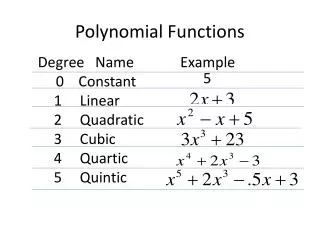
8. Polynomial Function Let  be a non-negative integer. A polynomial function is a function that can be written in the form This is called the general form of a polynomial function. Each  is a coefficient and can be any real number. Each product  is a term of a polynomial function.

9. Terminology of Polynomial Functions • We often rearrange polynomials so that the powers are descending • When a polynomial is written in this way, we say that it is in general form

10. End Behavior of Polynomial Functions For any polynomial, the end behavior of the polynomial will match the end behavior of the highest degree. In this example graph, the end behavior is: • as , • as , Therefore, this graph has the shape of anodd degree power function and theleading coefficient must be positive.

11. Identifying End Behavior and Degree of a Polynomial Function Describe the end behavior and determine a possible degree of the polynomial function in the graph below. As the input values  get very large, the output values  increase without bound. As the input values  get very small, the output values decrease without bound. We can describe the end behavior symbolically by writing We can tell this graph has the shape of an odd degree power function that has not been reflected, so the degree of the polynomial creating this graph must be odd and the leading coefficient must be positive.

12. Local Behavior of Polynomial Functions A turning point is a point at which the function values change from increasing to decreasing or decreasing to increasing. • The -intercept is the point at which the function has an input value of zero. • The -intercepts are the points at which the output value is zero. • A polynomial of degree  will have, at most, -intercepts and  turning points.

13. Principle of Zero Products The Principle of Zero Products states that if the product of n numbers is 0, then at least one of the factors is 0. If , then either or , or both and are 0. We will use this idea to find the zeros of a polynomial that is either in factored form, or can be written in factored form. For example, the polynomial is in factored form.

14. Intercepts of a Polynomial Function Use the factored form of a polynomial function to find it’s x and y-intercepts. The -intercept of a polynomial occurs when the input is zero. The -intercepts occur when the output is zero. Example: so the -intercept is at . when , , or (which has no real solution) so the -intercepts are at and .

15. Multiplicity If a polynomial contains a factor of the form , the behavior near the -intercept is determined by the power . We say that  is a zero of multiplicity.

16. How To: Given a Graph of a Polynomial Function of Degree , Identify Their Zeros and Their Multiplicities Given a graph of a polynomial function of degree , identify the zeros and their multiplicities. If the graph crosses the -axis and appears almost linear at the intercept, it is a single zero. If the graph touches the -axis and bounces off of the axis, it is a zero with even multiplicity. If the graph crosses the -axis at a zero, it is a zero with odd multiplicity. The sum of the multiplicities is .

17. Example: Identifying Zeros and Their Multiplicities Use the graph of the function of degree 6 to identify the zeros of the function and their possible multiplicities. The polynomial function is of degree . The sum of the multiplicities must be n. Starting from the left, the first zero occurs at . The graph touches the -axis, so the multiplicity of the zero must be even. The zero of –3 has multiplicity 2. The next zero occurs at . The graph looks almost linear at this point. This is a single zero of multiplicity 1. The last zero occurs at . The graph crosses the-axis, so the Multiplicityof the zero must be odd. We know that the multiplicity is likely 3 and that thesum of the multiplicities is likely 6.

18. Graphing Polynomial Functions • Find the intercepts • Check for symmetry. If the function is even, its graph is symmetrical about the -axis, that is, If a function is odd, its graph is symmetrical about the origin, • Use the multiplicities of the zeros to determine the behavior at the -intercepts • Determine the end behavior by examining the leading term • Use the end behavior and the behavior at the intercepts to sketch a graph • Ensure that the number of turning points does not exceed one less than the degree of the polynomial • Optionally, use technology to check the graph

19. Example: Sketching the Graph of a Polynomial Function • Sketch a graph of . This graph has two x-intercepts. At , the factor is squared, indicating a multiplicity of 2. The graph will bounce at this -intercept. At , the function has a multiplicity of one, indicating the graph will cross through the axis at this intercept. The -intercept is found by evaluating . The -intercept is . Additionally, we can see the leading term, if this polynomial were multiplied out, would be, so the end behavior is that of a vertically reflected cubic, with the outputs decreasing as the inputs approach infinity, and the outputs increasing as the inputs approach negative infinity.

20. Example: Sketching the Graph of a Polynomial Function

21. Intermediate Value Theorem TheIntermediate Value Theorem states that If and  have opposite signs, then there exists at least one value  between  and  for which 

22. Factored Form of Polynomials If a polynomial of lowest degree  has horizontal intercepts at  , then the polynomial can be written in the factored form: where the powers  on each factor can be determined by the behavior of the graph at the corresponding intercept, and the stretch factor  can be determined given a value of the function other than the -intercept.

23. Local and Global Extrema A local maximum or local minimum at is the output at the highest or lowest point on the graph in an open interval around  A global maximum or global minimum is the output at the highest or lowest point of the function. If a function has a global maximum at , then  for all . If a function has a global minimum at , then for all .

24. Desmos Interactive Topic: zeros from a graph with slider = a to change y-intercept https://www.desmos.com/calculator/5oyyx0vbiv

25. Division Algorithm The Division Algorithm states that, given a polynomial dividend  and a non-zero polynomial divisor  where the degree of  is less than or equal to the degree of , there exist unique polynomials  and  such that is the quotient and  is the remainder. The remainder is either equal to zero or has degree strictly less than  If, then  divides evenly into . This means that, in this case, both  and  are factors of .

26. Synthetic Division Synthetic division is a shortcut that can be used when the divisor is a binomial in the form . In synthetic division, only the coefficients are used in the division process

27. The Remainder Theorem If a polynomial  is divided by , then the remainder is the value . Given a polynomial function , evaluate at using the Remainder Theorem. • Use synthetic division to divide the polynomial by . • The remainder is the value . Example: Evaluate at . Use synthetic division: The remainder is 25. Therefore, .

28. The Rational Zero Theorem The Rational Zero Theorem states that, if the polynomial has integer coefficients, then every rational zero of  has the form  where  is a factor of the constant term and is a factor of the leading coefficient . When the leading coefficient is 1, the possible rational zeros are the factors of the constant term. Example: List all possible rational zeros of . Solution: The constant term is −4; the factors of −4 are ±1, ±2, and ±4. The leading coefficient is 2; the factors of 2 are ±1 and ±2. Therefore, any possible zeros are: ±1, ±2, ±4 and ±½.

29. The Factor Theorem The Factor Theorem states that is a zero of  if and only if  is a factor of . Given a factor and a third-degree polynomial, use the Factor Theorem to factor the polynomial. • Use synthetic division to divide the polynomial by . • Confirm that the remainder is 0. • Write the polynomial as the product of and the quadratic quotient. • If possible, factor the quadratic. • Write the polynomial as the product of factors.

30. Find Zeros of a Polynomial Function Given a polynomial function , use synthetic division to find its zeros. • Use the Rational Zero Theorem to list all possible rational zeros of the function. • Use synthetic division to evaluate a given possible zero by synthetically dividing the candidate into the polynomial. If the remainder is 0, the candidate is a zero. If the remainder is not zero, discard the candidate. • Repeat step two using the quotient found with synthetic division. If possible, continue until the quotient is a quadratic. • Find the zeros of the quadratic function. Two possible methods for solving quadratics are factoring and using the quadratic formula.

31. Fundamental Theorem of Algebra The Fundamental Theorem of Algebra states that, if is a Polynomial of Degree , then has at least one Complex Zero We can use this theorem to argue that, if  is a polynomial of degree , and  is a non-zero real number, then  has exactly  linear factors where  are complex numbers. Therefore,  has  roots if we allow for multiplicities.

32. Complex Conjugate Theorem According to the Linear Factorization Theorem, a polynomial function will have the same number of factors as its degree, and each factor will be in the form , where  is a complex number. If the polynomial function  has real coefficients and a complex zero in the form , then the complex conjugate of the zero, , is also a zero.

33. Descartes’ Rule of Signs According to Descartes’ Rule of Signs, if we let be a polynomial function with real coefficients: • The number of positive real zeros is either equal to the number of sign changes of  or is less than the number of sign changes by an even integer. • The number of negative real zeros is either equal to the number of sign changes of  or is less than the number of sign changes by an even integer.

34. Quick Review • What is a power function? • Is  a power function? • What does the end behavior depend on? • Do all polynomial functions have a global minimum or maximum? • What is synthetic division? • Does every polynomial have at least one imaginary zero? • If  were given as a zero of a polynomial with real coefficients, would also need to be a zero?