Download
1 / 16
160 likes | 321 Views
Generating Sinusoidal Signals. Prof. Brian L. Evans Dept. of Electrical and Computer Engineering The University of Texas at Austin. EE 445S Real-Time Digital Signal Processing Lab Fall 2014. Lecture 1 http://www.ece.utexas.edu/~bevans/courses/realtime. Outline.

E N D
Generating Sinusoidal Signals Prof. Brian L. Evans Dept. of Electrical and Computer Engineering The University of Texas at Austin EE 445S Real-Time Digital Signal Processing Lab Fall 2014 Lecture 1 http://www.ece.utexas.edu/~bevans/courses/realtime
Outline Bandwidth Sinusoidal amplitude modulation Sinusoidal generation Design tradeoffs
Bandwidth Ideal Bandpass Spectrum Ideal Lowpass Spectrum f f -fmax fmax –f1 f2 –f2 f1 Bandwidth W = f2 – f1 Bandwidth fmax Bandwidth • Non-zero extent in positive frequencies • Applies to continuous-time & discrete-time signals • In practice, spectrum won’t be ideally bandlimited Thermal noise has “flat” spectrum from 0 to 1015 Hz Finite observation time of signal leads to infinite bandwidth • Alternatives to “non-zero extent”?
Bandwidth Lowpass Signal in Noise • How to determine fmax? Apply threshold and eyeball it OR Estimate fmax that captures certainpercentage (say 90%) of energyIn practice, (a) use large frequency in place of and (b) integrate a measured spectrum numerically Lowpass Spectrum in Noise f Idealized Lowpass Spectrum approximate f -fmax fmax Baseband signal: energy in frequency domain concentrated around DC
Bandwidth Idealized Bandpass Spectrum f –f1 f2 –f2 f1 Bandpass Signal in Noise Bandpass Spectrum In Noise • How to find f1 and f2? Apply threshold and eyeball it OR Assume knowledge of fc andestimate f1 = fcW/2 andf2 = fc+ W/2 that capture percentage of energyIn practice, (a) use large frequency in place of and (b) integrate a measured spectrum numerically f - fc fc
Amplitude Modulation lower sidebands Y1(w) ½X1(w + wc) ½X1(w - wc) X1(w) ½ 1 w -wc - w1 -wc + w1 wc - w1 wc + w1 0 -wc wc w -w1 w1 0 Amplitude Modulation by Cosine • y1(t) = x1(t) cos(wct) Assume x1(t) is an ideal lowpass signal with bandwidth w1 Assume w1 << wc Y1(w) has (transmission) bandwidth of 2w1 Y1(w) is real-valued if X1(w) is real-valued • Demodulation: modulation then lowpass filtering
Amplitude Modulation Y2(w) j ½X2(w + wc) -j ½X2(w - wc) X2(w) j ½ 1 wc wc – w2 wc + w2 w -wc – w2 -wc + w2 -wc w -j ½ -w2 w2 0 Amplitude Modulation by Sine • y2(t) = x2(t) sin(wct) Assume x2(t) is an ideal lowpass signal with bandwidth w2 Assume w2 << wc Y2(w) has (transmission) bandwidth of 2w2 Y2(w) is imaginary-valued if X2(w) is real-valued • Demodulation: modulation then lowpass filtering lower sidebands
Amplitude Modulation How to Use Bandwidth Efficiently? • Send lowpass signals x1(t)and x2(t) with 1 = 2 oversame transmission bandwidth Called Quadrature Amplitude Modulation (QAM) Used in DSL, cable, Wi-Fi, andLTE cellular communications • Cosine modulated signal is in theory orthogonal to sine modulated signal at transmitter Receiver separates x1(t) and x2(t) through demodulation x1(t) s(t) cos(ct) + x2(t) sin(c t)
Sinusoidal Generation Lab 2: Sinusoidal Generation • Compute sinusoidal waveform Function call Lookup table Difference equation • Output waveform off chip Polling data transmit register Software interrupts Quantization effects in digital-to-analog (D/A) converter • Expected outcomes are to understand Signal quality vs. implementation complexity tradeoff Interrupt mechanisms
Design Tradeoffs in Generating Sinusoidal Signals Sinusoidal Waveforms • One-sided discrete-time cosine (or sine) signal with fixed-frequency 0 in rad/sample has form cos(0n) u[n] • Consider one-sided continuous-time analog-amplitude cosine of frequency f0 in Hz cos(2 f0t) u(t) Sample at rate fs by substituting t = nTs = n / fs (1/Ts) cos(2 (f0 / fs) n) u[n] Discrete-time frequency 0 = 2 f0 / fsin units of rad/sample Example: f0 = 1200 Hz and fs = 8000 Hz, 0 = 3/10 • How to determine gain for D/A conversion? See handout on sampling unit step function
Design Tradeoffs in Generating Sinusoidal Signals Math Library Call in C • Uses double-precision floating-point arithmetic • No standard in C for internal implementation • Appropriate for desktop computing On desktop computer, accuracy is a primary concern, so additional computation is often used in C math libraries In embedded scenarios, implementation resources generally at premium, so alternate methods are typically employed • GNU Scientific Library (GSL)cosine function Function gsl_sf_cos_e in file specfunc/trig.c Version 1.8 uses 11th order polynomial over 1/8 of period 20 multiply, 30 add, 2 divide and 2 power calculations per output value (additional operations to estimate error)
Design Tradeoffs in Generating Sinusoidal Signals Efficient Polynomial Implementation • Use 11th-order polynomial Direct form a11x11 + a10x10 + a9x9 + ... + a0 Horner's form minimizes number of multiplications a11x11 + a10x10 + a9x9 + ... + a0 = ( ... (((a11x + a10) x + a9) x ... ) + a0 • Comparison
Design Tradeoffs in Generating Sinusoidal Signals Difference Equation • Difference equation with input x[n] and output y[n] y[n] = (2 cos 0) y[n-1] - y[n-2] + x[n] - (cos 0) x[n-1] From inverse z-transform of z-transform of cos(0n) u[n] Impulse response gives cos(0n) u[n] Similar difference equation for sin(0n) u[n] • Implementation complexity Computation: 2 multiplications and 3 additions per cosine value Memory Usage: 2 coefficients, 2 previous values of y[n] and1 previous value of x[n] • Drawbacks Buildup in error as n increases due to feedback Fixed value for 0 Initial conditions are all zero
Design Tradeoffs in Generating Sinusoidal Signals Difference Equation • If implemented with exact precision coefficients and arithmetic, output would have perfect quality • Accuracy loss as n increases due to feedback from Coefficients cos(0) and 2 cos(0) are irrational, except when cos(0) is equal to -1, -1/2, 0, 1/2, and 1 Truncation/rounding of multiplication-addition results • Reboot filter after each period of samples by resetting filter to its initial state Reduce loss from truncating/rounding multiplication-addition Adapt/update 0 if desired by changing cos(0) and 2 cos(0)
Design Tradeoffs in Generating Sinusoidal Signals Lookup Table • Precompute samples offline and store them in table • Cosine frequency 0 = 2 N / L Remove all common factors between integers N and L Continuous-time period for cos(2 f0 t) is T0 = 1 / f0 Discrete-time period for cos(2 (N / L) n)is L samples Store L samples in lookup table (N continuous-time periods) • Built-in lookup tables in read-only memory (ROM) Samples of cos() and sin() at uniformly spaced values for Interpolate values to generate sinusoids of various frequencies Allows adaptation of 0 if desired
Design Tradeoffs in Generating Sinusoidal Signals Design Tradeoffs • Signal quality vs. implementation complexity in generating cos(0n) u[n] with 0 = 2 N / L MAC Multiplication-accumulationRAM Random Access Memory (writeable) ROM Read-Only Memory