Attribute Grammar
Attribute Grammar. Professor Yihjia Tsai Tamkang University. Action Routines and Attribute Grammars. Automatic tools can construct lexer and parser for a given context-free grammar E.g. JavaCC and JLex/CUP (and Lex/Yacc ) CFGs cannot describe all of the syntax of programming languages

Attribute Grammar
E N D
Presentation Transcript
Attribute Grammar Professor Yihjia Tsai Tamkang University
Action Routines and Attribute Grammars • Automatic tools can construct lexer and parser for a given context-free grammar • E.g. JavaCC and JLex/CUP (and Lex/Yacc) • CFGs cannot describe all of the syntax of programming languages • An ad hoc techniques is to annotate the grammar with executable rules • These rules are known as action routines • Action routines can be formalized Attribute Grammars • Primary value of AGs: • Static semantics specification • Compiler design (static semantics checking)
Attribute Grammars • Example: expressions of the form id + id • id's can be either int_type or real_type • types of the two id's must be the same • type of the expression must match it's expected type • BNF: <expr> <var> + <var> <var> id • Attributes: • actual_type - synthesized for <var> and <expr> • expected_type - inherited for <expr>
The Attribute Grammar • Syntax rule: <expr> <var>[1] + <var>[2] Semantic rules: <expr>.actual_type <var>[1].actual_type Predicate: <var>[1].actual_type == <var>[2].actual_type <expr>.expected_type == <expr>.actual_type • Syntax rule: <var> id Semantic rule: <var>.actual_type lookup (<var>.string)
Attribute Grammars <expr>.expected_type inherited from parent <var>[1].actual_type lookup (A) <var>[2].actual_type lookup (B) <var>[1].actual_type =? <var>[2].actual_type <expr>.actual_type <var>[1].actual_type <expr>.actual_type =? <expr>.expected_type
Attribute Grammars • Def: An attribute grammar is a CFG G = (S, N, T, P) with the following additions: • For each grammar symbol x there is a set A(x) of attribute values • Each rule has a set of functions that define certain attributes of the nonterminals in the rule • Each rule has a (possibly empty) set of predicates to check for attribute consistency
Attribute Grammars • Let X0 X1 ... Xn be a rule • Functions of the form S(X0) = f(A(X1), ... , A(Xn)) define synthesized attributes • Functions of the form I(Xj) = f(A(X0), ... , A(Xn)), for i <= j <= n, define inherited attributes • Initially, there are intrinsic attributes on the leaves
Attribute Grammars • How are attribute values computed? • If all attributes were inherited, the tree could be decorated in top-down order. • If all attributes were synthesized, the tree could be decorated in bottom-up order. • In many cases, both kinds of attributes are used, and it is some combination of top-down and bottom-up that must be used. • Top-down grammars (LL(k)) generally require inherited flows
Attribute Grammars and Practice • The attribute grammar formalism is important • Succinctly makes many points clear • Sets the stage for actual, ad-hoc practice • The problems with attribute grammars motivate practice • Non-local computation • Need for centralized information (globals) • Advantages • Addresses the shortcomings of the AG paradigm • Efficient, flexible • Disadvantages • Must write the code with little assistance • Programmer deals directly with the details
The Realist’s Alternative Ad-hoc syntax-directed translation • Associate a snippet of code with each production • At each reduction, the corresponding snippet runs • Allowing arbitrary code provides complete flexibility • Includes ability to do tasteless & bad things To make this work • Need names for attributes of each symbol on lhs & rhs • Typically, one attribute passed through parser + arbitrary code (structures, globals, statics, …) • Yacc/CUP introduces $$, $1, $2, … $n, left to right • Need an evaluation scheme • Fits nicely into LR(1)parsing algorithm
Generation of parsers • We have seen that recursive decent parsers can be constructed automatically, e.g. JavaCC • However, recursive decent parsers only work for LL(k) grammars • Sometimes we need a more powerful language • The LR languages are more powerful • Parsers for LR languages a use bottom-up parsing strategy
Sentence Subject Object Noun Verb Noun Bottom up parsing The parse tree “grows” from the bottom (leafs) up to the top (root). The The cat cat sees sees a a rat rat . .
Bottom Up Parsers • Harder to implement than LL parser • but tools exist (e.g. JavaCUP and SableCC) • Can recognize LR0, LR1, SLR, LALR grammars (bigger class of grammars than LL) • Can handle left recursion! • Usually more convenient because less need to rewrite the grammar. • LR parsing methods are the most commonly used for automatic tools today (LALR in particular)
Bottom Up Parsers: Overview of Algorithms • LR0 : The simplest algorithm, theoretically important but rather weak (not practical) • SLR : An improved version of LR0 more practical but still rather weak. • LR1 : LR0 algorithm with extra lookahead token. • very powerful algorithm. Not often used because of large memory requirements (very big parsing tables) • LALR : “Watered down” version of LR1 • still very powerful, but has much smaller parsing tables • most commonly used algorithm today
Fundamental idea • Read through every construction and recognize the construction in the end • LR: • Left – the string is read from left to right • Right – we get a right derivation • The parse tree is build from bottom up
Right derivations Sentence Subject Verb Object . Subject Verb a Noun . Subject Verb a rat . Subject sees a rat . The Noun sees a rat . The cat sees a rat . Sentence ::= Subject Verb Object . Subject ::= I | aNoun | theNoun Object ::= me | aNoun | the Noun Noun ::= cat | mat| rat Verb ::= like| is | see | sees
Sentence Subject Object Noun Verb Noun Bottom up parsing The parse tree “grows” from the bottom (leafs) up to the top (root). Just read the right derivations backwards The The cat cat sees sees a a rat rat . .
Bottom Up Parsers • All bottom up parsers have similar algorithm: • A loop with these parts: • try to find the leftmost node of the parse tree which has not yet been constructed, but all of whose children have been constructed. (This sequence of children is called a handle) • construct a new parse tree node. This is called reducing • The difference between different algorithms is only in the way they find a handle.
Bottom-up Parsing • Intuition about handles: • Def: is the handle of the right sentential form = w if and only if S =>*rm Aw =>rm w • Def: is a phrase of the right sentential form if and only if S =>* = 1A2=>+ 12 • Def: is a simple phrase of the right sentential form if and only if S =>* = 1A2=> 12
Bottom-up Parsing • Intuition about handles: • The handle of a right sentential form is its leftmost simple phrase • Given a parse tree, it is now easy to find the handle • Parsing can be thought of as handle pruning
Bottom-up Parsing • Shift-Reduce Algorithms • Reduce is the action of replacing the handle on the top of the parse stack with its corresponding LHS • Shift is the action of moving the next token to the top of the parse stack
The LR-parse algorithm • A finite automaton • With transitions and states • A stack • with objects (symbol, state) • A parse table
Model of an LR parser: input a1 … a2 … an $ Sm xm … s1 x1 s0 LR parsing program output Parsing table Action goto stack si is a state, xi is a grammar symbol All LR parsers use the same algorithm, different grammars have different parsing table.
The parse table • For every state and every terminal • either shift x Put next input-symbol on the stack and go to state x • or reduce production On the stack we now have symbols to go backwards in the production – afterwards do a goto • For every state and every non-terminal • Goto x Tells us, in which state to be in after a reduce-operation • Empty cells in the table indicates an error
Example-grammar • (0) S’ S$ • This production augments thegrammar • (1) S (S)S • (2) S • This grammar generates all expressions of matching parentheses
Example - parse table By reduce we indicate the number of the production r0 = accept Never a goto by S'
Example – parsing Stack Input Action $0 ()()$ shift 2 $0(2 )()$ reduce S $0(2S3 )()$ shift 4 $0(2S3)4 ()$ shift 2 $0(2S3)4(2 )$ reduce S $0(2S3)4(2S3 )$ shift 4 $0(2S3)4(2S3)4 $ reduce S $0(2S3)4(2S3)4S5 $ reduce S(S)S $0(2S3)4S5 $ reduce S(S)S $0S1 $ reduce S’S
The resultat • Read the productions backwards and we get a right derivation: • S’ S (S)S (S)(S)S (S)(S) (S)() ()()
LR(0)-items Item : A production with a selected position (marked by a point) X . indicates that at the stack we have and the first of the input can be derived from Our example grammar has the following items: S’ .S$ S’ S.$ (S’ S$.) S .(S)S S(.S)S S(S.)S S(S).S S(S)S. S.
LR(0)-DFA • Every state is a set of items • Transitions are labeled by symbols • States must be closed • New states are constructed from states and transitions
Closure(I) Closure(I) = repeat for any item A.X in I for any production X I I { X. } unto I does not change return I
Goto(I,X) Describes the X-transition from the state I Goto(I,X) = Set J to the empty set for any item A.X in I add AX. to J return Closure(J)
LR(0)-parse table • state I with x-transition (x terminal) to J • shift J in cell (I,x) • state I with final item ( X. ) corresponding to the productionen n • reduce n in all celler (I,x) for all terminals x • state I with X-transition (x non-terminal) to J • goto J in cell (I,X) • empty cells - error
Shift-reduce-conflicts • What happens, if there is a shift and a reduce in the same cell • so we have a shift-reduce-conflict • and the grammar is not LR(0) • Our example grammar is not LR(0)
LR0 Conflicts The LR0 algorithm doesn’t always work. Sometimes there are “problems” with the grammar causing LR0 conflicts.An LR0 conflict is a situation (DFA state) in which there is more than one possible action for the algorithm. • More precisely there are two kinds of conflicts: • shift <-> reduce • When the algorithm cannot decide between a shift action or • a reduce action • reduce <-> reduce • When the algorithm cannot decide between two (or more) reductions (for different grammar rules).
Parser Conflict Resolution Most programming language grammars are LR 1. But, in practice, one still encounters grammars which have parsing conflicts. => a common cause is an ambiguous grammar Ambiguous grammars always have parsing conflicts (because they are ambiguous this is just unavoidable). In practice, parser generators still generate a parser for such grammars, using a “resolution rule” to resolve parsing conflicts deterministically. => The resolution rule may or may not do what you want/expect => You will get a warning message. If you know what you are doing this can be ignored. Otherwise => try to solve the conflict by disambiguating the grammar.
Parser Conflict Resolution Example: (from Mini-triangle grammar) single-Command ::= ifExpression thensingle-Command | ifExpression thensingle-Command elsesingle-Command This parse tree? single-Command single-Command ifa thenifb thenc1 elsec2
Parser Conflict Resolution Example: (from Mini-triangle grammar) single-Command ::= ifExpression thensingle-Command | ifExpression thensingle-Command elsesingle-Command or this one ? single-Command single-Command ifa thenifb thenc1 elsec2
Parser Conflict Resolution Example: “dangling-else” problem (from Mini-triangle grammar) single-Command ::= ifExpression thensingle-Command | ifExpression thensingle-Command elsesingle-Command LR1 items (in some state of the parser) sC ::= ifE thensC • {… else …} sC ::= ifE thensC • else sC {…} Shift-reduceconflict! Resolution rule: shift has priority over reduce. Q: Does this resolution rule solve the conflict? What is its effect on the parse tree?
Parser Conflict Resolution There is usually also a resolution rule for shift-reduce conflicts, for example the rule which appears first in the grammar description has priority. Reduce-reduce conflicts usually mean there is a real problem with your grammar. => You need to fix it! Don’t rely on the resolution rule!
LR(0) vs. SLR • LR(0) - here we do not look at the next symbol in the input before we decide whether to shift or to reduce • SLR - here we do look at the next symbol • reduce X is only necessary, when the next terminal y is in follow(X) • this rule removes at lot of potential s/r- og r/r-conflicts
SLR • DFA as the LR(0)-DFA • the parse table is a bit different: • shift and goto as with LR(0) • reduce X only in cells (X,w) with wfollow(X) • this means fewer reduce-actions and so fewer conflicts
LR(1) • Items are now pairs (A. , x) • x is an arbitrary terminal • means, that the top of the stack is and the input can be derivered from x • Closure-operation is different • Goto is (more or less) the same • The initial state is generated from (S' .S$, ?)
LR(1)-the parse table • Shift and goto as before • Reduce • state I with item (A., z) gives a reduce A in cell (I,z) • LR(1)-parse tables are very big
Example 0: S' S$ 1: S V=E 2: S E 3: E V 4: V x 5: V *E