The Pollution-Climate Connection
180 likes | 204 Views
This study examines the potential impact of climate change on pollution episodes in the United States. It explores the relationship between temperature, chemical reactions, atmospheric conditions, and pollution severity. The findings highlight the need for further research in order to better understand and address the complex interactions between climate change and pollution.

The Pollution-Climate Connection
E N D
Presentation Transcript
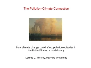
The Pollution-Climate Connection How climate change could affect pollution episodes in the United States: a model study Loretta J. Mickley, Harvard University
Number of summer days with 8-hour ozone > 84 ppbv, average for northeast U.S. sites Probability of ozone exceedance vs. daily max. temperature 1988, hottest on record Lin et al. 2001 We know that day-to-day meteorology affects the severity and duration of pollution episodes. New England days Why does probability of ozone episode increase with increasing temperature? Faster chemical reactions, increased biogenic emissions, and stagnation.
Top of boundary layer ozone, aerosol strong mixing How will a changing climate affect pollution? Answer: we don’t know. Rising temperatures could mean faster chemical reactions. . . Higher surface temperatures could also mean a deeper boundary layer, diluting concentrations at the surface. The picture is complicated, and the answer matters. { Soup of pollution precursors
Need sunlight, water vapor, and a mix of manmade or natural “ingredients.” How to make pollution: H2O Hydroxyl (OH) winds + Ozone (O3) Nitrogen oxides CO, Hydrocarbons rainout (important for aerosols) deposition Fires Biosphere Human activity Our approach: focus on changes in winds and rainout.
Pilot Project: Implement “tracers of anthropogenic pollution” into GISS General Circulation Model Goddard Institute for Space Studies GCM: 9 layers, 4ox5o horizontal grid, CO2 + other greenhouse gases increased yearly from 2000 to 2050. Carbon Monoxide: COt source: present-day manmade emissions sink: CO + present-day OH fields Black Carbon: BCt source: present-day manmade emissions sink: rainout July global mean temperature 2045-2052 +2o C Temp change { spin up 1995-2002 Sensitive to climate change Circulationalso sensitive to climate change Timeline 1950 spin-up (ocean adjusts) 2000 increasing A1 greenhouse gas 2050
midwest northeast California southeast Our approach: Look at daily mean concentrations averaged over specific regions for two 8-year intervals (1995-2002) and (2045-2052). Histogram of COt concentrations averaged over Northeast for 1995-2002 summers (July-Aug) Cumulative probability plotshows the percentage of points below a certain concentration. Note: concentrations are low compared to observations since only source is direct manmade emissions.
Frequency distributions for surface COt and BCt show significantly higher extremes in 2050s compared to present-day. July - August 2045-2052 1995-2002 Changes at the extremes are due solely to changes in circulation and rainfall.
Frequency distributions for three U.S. regions in July-August show increased severity of pollution episodes. 2050 2000 In all regions, daily COt and BCt concentrations correlate (R2 ~ 0.6 – 0.8) so changes are likely due to circulation.
How does depth of boundary layer change with changing climate? Northeast daily maximum boundary layer height. Triangles indicate days of high pollution. Extreme pollution events associated with lower boundary layer heights. Higher BL heights in future go in opposite direction to what is needed to explain air quality differences. 2045-2052 1995-2002
Evolution of a typical pollution event. This happens repeatedly during summertime. cyclone (low pressure system) weak winds BCt and wind fields for 6 consecutive days in summer. cold front from Canada 100 x mg/m3
Is pollution more persistent in future? How often do cold fronts come through to sweep away pollution? Mean frequency of cold fronts pushing into Midwest decreases by ~20% in future climate. Persistence of pollution episodes increases by 30-100% over Midwest. Cyclone number and cold front frequency decline in future, allowing pollutants to build up.
A decrease in cyclone frequency over midlatitudes has also been observed in recent decades. 1000 cyclones Agee, 1991 annual number of surface cyclones and anticylones for North America and nearby ocean 500 100 anticyclones 1950 1980 McCabe et al., 2001 Standardized departure of cyclone frequency over Northern Hemisphere. 30-60N Other model studies of future climatehave found similar declines relative to the present-day.
Two mechanisms for the meridional transport of energy on a round, wet world. 1. Mid-latitude cyclones push warm air poleward ahead of front, push cold air equatorward behind front. warm tropics cold poles cold front 2. Eddy transport of latent heat carries energy to higher latitudes.
Reasons for decline in cyclone generation over midlatitudes. Change in zonally averaged temperature for July-August. Increase is greatest at high latitudes. Reason is ice-albedo feedback. DT Change in northward transport of latent heat by eddies in mid-troposphere in future atmosphere. Reduced temperature gradient and more efficient eddy transport of energy poleward Fewer cyclones generated More persistent pollution events
2050 2000 Reduced cloud cover How do you translate our results into “ozone alert days”? Model predicts high-pollution days will occur about 66% more frequently in future due to changes in circulation over Northeast and Midwest. Best calculation includes full chemistry responding to all the meteorological changes. Hotter maximum temperatures Triangles indicate days of highest BCt concentrations. High maximum temperatures and reduced cloud cover suggest increased ozone production, amplifying effect of stagnation.
Monitoring pollution and biomass burning over North America with satellites AIRS instrument onboard the AQUA satellite enables observation of complex and overlapping long-range transport. AIRS COColumn July 18, 2004 GEOS-CHEM COColumn July 18, 2004 model fires Asian pollution U.S. pollution Wallace McMillan (UMBC) Solene Turquety (Harvard)
First day of ozone column data from TES TES = Tropospheric Emission Spectrometer Measures infrared radiances in both limb and nadir mode. Launched July 15, 2004 Will provide a detailed, global view of ozone, CO, and HNO3 First day of data! Tropospheric ozone column on September 20, 2004 pollution pollution biomass burning
Summary Model predicts an increase in the severity and duration of pollution episodes over the Midwest and Northeast U.S. by 2050, even with constant emissions. Change in pollution tied to a decrease in the frequency of cold fronts arriving from Canada, which sweep away the pollution. 2050s Observed correlations between meteorological parameters and pollutant concentrations provide a tool for predicting trends in GCM simulations. A new era of satellite observations probing the troposphere can supply data to assess our model predictions. 2000s