Understanding the Multinomial Distribution: Concepts, Applications, and Hypothesis Testing
This comprehensive guide explores the multinomial distribution, focusing on its definition, coefficients, and the maximum likelihood estimation. We examine its application through examples, such as determining employment outcomes for graduating students, and discuss hypothesis testing, including large-sample likelihood ratio tests. The multinomial distribution's role in statistical experimentation, marginal probabilities, and multivariate distributions are also covered. Gain insights into estimating probabilities, expected values, and how the central limit theorem applies in this context.

Understanding the Multinomial Distribution: Concepts, Applications, and Hypothesis Testing
E N D
Presentation Transcript
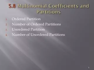
Multinomial Distribution • Multinomial coefficients • Definition • Marginals are binomial • Maximum likelihood • Hypothesis tests
Multinomial Coefficient: From n objects, number of ways to choose • n1 of type 1 • n2 of type 2 • nk of type k
Of 30 graduating students, how many ways are there for 15 to be employed in a job related to their field of study, 10 to be employed in a job unrelated to their field of study, and 5 unemployed?
Multinomial Distribution • Statistical experiment with k outcomes • Repeated independently n times • Pr(Outcome j) = pj, j = 1, …, k • Number of times outcome j occurred is xj, j = 1, …, k • A multivariate distribution
Observe • Adding over xk-1 throws it into the “leftover” category. • Labels 1, …, k are arbitrary, so this means you can combine any 2 categories and the result is still multinomial. • k is arbitrary, so you can keep doing it and combine any number of categories. • When only two categories are left, the result is binomial • E(xj) = npj, Var(xj) = npj(1-pj)
Sample problem • P(Job related to field of study) = 0.60 • P(Job unrelated to field of study) = 0.30 • P(No job) = 0.10 • Of 30 randomly chosen students, what is probability that 15 are employed in a job related to their field of study, 10 are employed in a job unrelated to their field of study, and 5 are unemployed? • What is the probability that exactly 5 are unemployed?
Lessons from the data file • Cases (N of them) are independent M(1,p), so E(xi,j) = pj. • Column totals count the number of times each category occurs: Joint distribution is M(N,p) • These are the table (cell) frequencies! They are random variables, and now we know their joint distribution. • Each individual table frequency is B(N,pj) • Expected value of frequency j is mj = Npj • Tables of 2 and or more dimensions present no problems -- combination variables.
More about the frequencies We are in the familiar situation of estimating expected values with sample means. And these sample means are just sample proportions.
Simple Tools for Estimation • So the (multivariate) sample mean is an unbiased estimator of the vector of multinomial probabilities. • The Law of Large numbers says • CLT says multivariate sample mean has an approximate multivariate normal distribution for large N. • Basis of large-sample tests and confidence intervals.
Maximum Likelihood • Product of N probability mass functions, each • M(1,p) • Depends upon the sample data only through the vector of k frequency counts. • By the factorization theorem, a sufficient statistic • All the information about the parameter in the sample data is contained in the sufficient statistic.
Following the book’s notation • Write the frequencies as x1, …, xk. • Later, x values with multiple subscripts will refer to frequencies in a multi-dimensional table, like xi,j,k will be the frequency in row i and column j of sub-table k. • Write likelihood function as
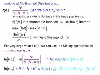
Log likelihood: p-1 parameters Set all k-1 derivatives to zero and solve for p1, …, pk. Verify that pi = xi /N for i = 1, … k–1 works: MLE is the sample mean.
Likelihood Ratio Tests Under H0, G2 has an approximate chi-square distribution for large N. Degrees of freedom = number of (non-redundant, linear) equalities specified by H0. Reject when G2 is large.
Degrees of Freedom • Express H0 as a set of linear combinations of the parameters, set equal to constants (usually zeros). • Degrees of freedom = number of non-redundant linear combinations. df=3
p = (p1,p2,p3,p4,p5) • H0: p1=0.25, p2=(p3+p4)/2,p4=p5 so df=3 • H0: p1=1/5, p2=1/5, p3=1/5, p4=1/5, p5=1/5 so df=4 not 5, because probabilities add to one, so one equality is redundant. If is a kx1 vector and H0: C = h where C is an rxk matrix, the degrees of freedom is the row rank (number of linearly independent rows) of C --- usually r. But remember, if = p for the multinomial, there are really k-1 parameters.
Example University administrators recognize that the percentage of students who are unemployed after graduation will vary depending upon economic conditions, but they claim that still, about twice as many students will be employed in a job related to their field of study, compared to those who get an unrelated job. To test this hypothesis, they select a random sample of 200 students from the most recent class, and observe 106 employed in a job related to their field of study, 74 employed in a job unrelated to their field of study, and 20 unemployed. Test the hypothesis using a large-sample likelihood ratio test and significance level = 0.05. State your conclusions in symbols and words.
What is the model? • What is the null hypothesis, in symbols? • What are the degrees of freedom for this test?
What is the restricted MLE? Your answer is a symbolic expression. It’s a vector. Show your work.
What is the unrestricted MLE? Your answer is a numeric vector: 3 numbers. • What is the restricted MLE? Your answer is a numeric vector: 3 numbers. • What are the estimated expected frequencies under the null hypothesis? Your answer is a numeric vector: 3 numbers.
State your conclusions • In symbols: Reject H0: p1=2p2 at alpha = 0.05 • In words: More graduates appear to be employed in jobs unrelated to their fields of study than expected. Statement in words is justified because Observed 106 74 20 Expected 120 60 20 Obs-Exp -14 14 0
Two chi-square formulas • Likelihood Ratio • Pearson • Summation is over all cells • By expected frequency, we mean estimated expected frequency. • Asymptotically equivalent • Same degrees of freedom • Book's formula for df applies only to log-linear models. Use the approach given here, for now.
Pearson Chi-square on the jobs data Observed 106 74 20 Expected 120 60 20