15-853:Algorithms in the Real World

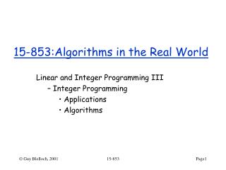
1. 15-853:Algorithms in the Real World Satisfiability Solvers (Lectures 1 & 2)

2. Satisfiability (SAT) The “original” NP-Complete Problem. • Input: Variables V = {x1, x2, …, xn}, Boolean Formula Φ (typically in conjunctive normal form (CNF)). e.g., Φ = (x1 v x2 v ¬x3) & (¬x1 v ¬x2 v x3) & … • Output: Either a satisfying assignment f:V → {True, False} that makes Φ evaluate to True, OR “Unsatisfiable” if no such assignment exists.

3. Extensions/Related Problems • Satisfiability Modulo Theories Input: a formula Φ in quantifier-free first-order logic. Output: is Φ satisfiable? • Theorem Provers • Pseudo-boolean optimization • Planners (Quantified SAT Solvers)

4. Applications • Verification: • Hardware: Electronic design automation market is about $6 Billion • Protocols: e.g., use temporal logic to reason about concurrency • Software • Optimization • Competitor to Integer Programming solutions in some domains • Math: Prove conjectures in finite algebra

5. An Aside: Example Proof by Machine • Thm: Robbins Algebra = Boolean Algebra • Robbins Algebra: values {0,1} and 3 axioms: x v (y v z) = (x v y) v z x v y = y v z ¬ (¬(x v y) v ¬(x v ¬y)) = x • Conjectured in 1933 • Proved in 1996 by prover EQP running for 8 days (RS/6000 with ~30 MB RAM) • Limited success since 1990s.

6. Annual Competitions • SAT Competition • CADE ATP System Competition • ASP Solver Competition • SMT-COMP • Constraint Satisfaction Solver Competition • Competitition/Exhibition of Termination Tools • TANCS • QBF Solvers Evaluation • Open Source Solvers: SATLIB, SATLive

7. Algorithms for SAT • Complete (satisfying assignment or UNSAT) • Davis-Putnam-Logemann-Loveland algorithm (DPLL) • Incomplete (satisfying assignment or FAILURE) • GSAT • WalkSAT

8. Prerequisite: Proof Systems • What constitutes a proof of unsatisfiability? • For a language L in {0,1}*, a proof system for membership in L is a poly-time computable function P such that • For all x in L, there is a witness y with P(x,y) = 1 • For all x not in L, for all y, P(x,y) = 0 • Complexity: worst case length of shortest witness for an x in L.

9. Proof System Examples • L = satisfiable boolean formulae • What’s the lowest complexity proof system for this you can come up with? • What about for L = unsatisfiable boolean formulae?

10. Proof System Examples • For unsatisfiability: • Witness = truth table T of Φ • P(Φ, T) checks that T is indeed the truth table for Φ, and all entries are zero • Corresponds to a (failed) brute force search for a solution • Exponential Complexity • Is there a proof system for UNSAT with poly complexity? (Does NP = Co-NP?)

11. Resolution Proof System • The Resolution Rule: • Witness = a sequence of valid derivations starting from the clauses of Φ. • Sound: (B v x) & (C v ¬x) implies (B v C) • Completefor unsatisfiability: • Every unsatisfiable formula has a derivation of a contradiction (i.e., the empty clause). For clauses B, C and variable x, From (B v x) & (C v ¬x) derive (B v C)

12. Duality • Truth table proof system gives proofs by failed search for a satisfying assignment. • Resolution proof system gives proofs by showing the initial clauses (constraints) yield a contradiction. This is a systematic search for additional constraints the solution must satisfy.

13. High level idea for many solvers • Alternate search for solution with search for properties of any solution: • Search for solution in some small part S of the space • If search in S fails, search for a reason for this failure, in the form of a new constraint C the solution must satisfy. • Search for a solution in a new part of the space, using new constraint to help guide the search • Repeat

14. Notation • Convenient notational change for SAT: • Clauses are sets: (a v ¬b v c) becomes {a, ¬b, c} • Formulae become sets of clauses • Partial assignments become sets of literals that contain at most one of {xi, ¬xi} for each i. • Assignments contain exactly one of {xi, ¬xi} for each i. • Restriction: Φ|{x} is the residual formula under partial assignment {x}, e.g., {{a, ¬b, c}, {¬a, b, d}} |{¬a} = {{¬b, c}}

15. Basic DPLL (‘60, ‘62) • Simple tree search for a solution, guided by the clauses of Φ. DPLL-recursive(formula F, partial assignment p) (F,p) = Unit-Propagate(F, p); If F contains clause {} then return (UNSAT, null); If F = {} then return (SAT, p); x = literal such that x and ¬x are not in p; (status, p’) = DPLL-recursive(F|{x}, pU{x}); If status == SAT then return (SAT, p’); Else return DPLL-recursive(F|{¬x}, pU{¬x}); If a clause tells you the value of a var, set it appropriately. Choose a branch. Many heuristics to choose from.

16. Basic DPLL If a clause tells you the value of a variable, set it appropriately. Unit-Propagate(formula F, partial assignment p) If F has no empty clause then While F has a unit clause {x} F = F|{x}; p = p U {x}; return (F,p)

17. Embellishing DPLL • Branch Selection Heuristics • Clause Learning • Backjumping heuristics • Watched literals • Randomized Restarts • Symmetry breaking • More powerful proof systems • …

18. Branch Selection Heuristics • Random • Max occurrence in clauses of min size • Max occurrence in as yet unsatisfied clauses • With probability proportional to some function of how often the literal appears in partial assignments that lead to unsatisfiable restricted formulae. • …

19. Clause Learning • When DPLL discovers F|p is unsatisfiable, it derives (learns) a reason for this in the form of new clauses to add to F. • What clauses are learned, and how, make huge differences in performance. • Trivially learned clause: if F|p is unsatisfiable for p = {x1, x2, …, xk}, derive clause {¬x1, ¬x2, …, ¬xk} But we want short clauses that constrain the solution space as much as possible…

20. Clause Learning • Use the clauses to guide the search: • So far we’ve seen unit-propagation, and search with restriction. • We want to learn clauses that let us prune effectively – this requires us to deduce “higher level” reasons why some partial assignment is no good. • Use resolution (or some technique) to try to prove that F|p is unsatisfiable for nodes p high up the tree.

21. High level: DPLL w/Clause Learning DPLL-CL (formula F) p = {} While(true) Choose a literal x such that x and ¬x are not in p; p = pU{x}; Deduce status from (F, p); // SAT, UNSAT, or unknown If status == SAT then return (SAT, p); If status == UNSAT then Analyze-Conflict(p); // Add learned clause(s) to F if p = {} then return (UNSAT, null); Else backtrack; // remove literals from p // based on learned clause(s) If status == unknown then continue; // branch again

22. Deduce • Tradeoff between searching more partial assignments (going deeper in the tree), and searching for proofs of unsatisfiability higher up in the tree. • Currently, deduction is typically just iterated unit-propagation. (Other embellishments to DPLL seem to render more complex deduction unhelpful in practice.)

23. Analyze Conflict: Implication Graph p = {¬x1, x3 , ¬x4} F = {{x1, x5}, {¬x3,x4, ¬x5}} {x1, x5} ¬x1 x5 {¬x3,x4, ¬x5} {¬x3,x4, ¬x5} x4 x3 conflict conflict ¬x4 From p

24. Implication Graph May contain several sources of conflicts. x6 ¬x1 x5 x4 ¬x7 x2 ¬x6 ¬x8 x3 ¬x5

25. Implication Graph The conflict graph for conflict variable x5 (solid edges). x6 ¬x1 x5 x4 ¬x7 x2 ¬x6 ¬x8 x3 ¬x5

26. Conflict Graphs The conflict graph for conflict variable x6 (solid edges). x6 ¬x1 x5 x4 ¬x7 x2 ¬x6 ¬x8 x3 ¬x5

27. Analyze Conflict Every nontrivial cut of each conflict graph yields a conflict clause. Which one(s) do we add to the clause set? {x1, ¬x3 , x4} {¬x3 , x4, ¬x5} ¬x1 x5 the trivial cut (not useful) x4 x3 conflict ¬x4

28. What Clauses to Learn? • Can’t keep everything -- space is a major bottleneck in practice. • Various heuristics: • First unique implication point • First new cut • Decision cut • …

29. Backtracking/Backjumping • For each x in p, maintain: • Int depth(x): number of literals in p immediately after x was added to p. • Bool flipped(x): did we try the partial assignment with ¬x and all literals at lower depth than x in p? • If we can derive a conflict clause C containing only x and literals of lower depth in p, then we can backtrack to x: • delete all literals with depth > depth(x) from p, • If flipped(x) = true, then delete x as well. • Other heuristics backtrack more aggressively.

30. Random Restarts • Restart: keep learned clauses, but throw away p, resample random bits, and start again. • Essentially a very aggressive backjump. • Can help performance a lot. • Run time distributions appear to be heavy-tailed.

32. Random Restarts: Heuristics • Fixed cutoff (always restart after T seconds) • Cutoff after k restarts is some function f(k) • Luby et. al. universal restart strategy for f(k) • f(k) = c*k, c^k, … • Restart policies based on predictive models of solver behavior: • Bayesian approaches, Dynamic Programming, • Online submodular function maximization*

33. Embellishing DPLL • Branch Selection Heuristics • Clause Learning • Backjumping heuristics • Watched literals • Randomized Restarts • Symmetry breaking • More powerful proof systems • …

34. Watched Literals • Clever lazy data structure Maintain two literals {x,y} per active clause C that are not set to false. (“C watches x,y”) • If x set to true, do nothing • If x set to false, • For each C watching x, • either find another variable for C to watch, • or do unit-propagation on C as appropriate. • For each previously active C’ containing ¬x, • set C’ to watch ¬x • If x is unset, do nothing (!)

35. Watched Literals • Helps quickly find if a clause is satisfied (just look at its watched literals) • Helps quickly identify clauses ripe for unit-propagation. • “now a standard method used by most SAT solvers for efficient constraint propagation” – Gomes et. al. “Satisfiability Solvers” • Partially explains why deduce step is typically just iterated unit-propagation

36. Symmetry Breaking • Symmetry is common in practice (e.g., identical trucks in vehicle routing) • SAT encoding throws away this info. • Symmetry is useful for some proofs: • e.g., Pigeon-hole principle: Impossible to place (n+1) birds into n bins, such that each bin gets at most one bird.

37. Pigeon Hole Principle • Exponentially long proofs via resolution. • Polynomially long proofs via cutting planes Binary var x(i,j) = assign bird i to bin j. 1) Each bird i gets a bin: ∑(bins j) x(i,j) = 1 2) Each bin j has capacity one: ∑(birds i) x(i,j) ≤ 1 Summing (1) over birds: ∑(birds i)∑(bins j) x(i,j) = n+1 Summing (2) over bins: ∑(bins j)∑(birds i) x(i,j) ≤ n Combine these to get 0 ≤ -1.

38. Symmetry Breaking • Symmetries provided as part of input, or automatically detected (typically via graph isomorphism) • Impose lexicographically minimal constraints • Simple case: If {xi : i = 1,2,…, k} are all interchangeable, add constraints (xi v ¬xj) for all i < j. “If there’s a solution with r of k vars set true, let them be x1 through xr”

39. Symmetry Breaking • Order the variables, imagine assignment as a vector x. • Identify permutations π on variables, such that if p is a satisfying assignment, then p•π is. • Add constraints x ≤ xπ Example: π = (2, 1, 3) x xπ

40. Other Proof Systems • Truth Tables • Frege Systems (includes resolution as a special case) • Extended Resolution: Add new vars • Resolution w/symmetry detection • Geometric systems (infer cutting planes) • …

41. Incomplete Algorithms • Returns satisfying assignment or FAILURE • Based on heuristic search for a solution • Faster than complete algorithms for many classes of satisfiable instances. • Examples: • GSAT, WalkSAT, • Survey Propagation/Belief Propagation • Local search algs, Simulated Annealing, ILP, …

42. Greedy-SAT • GSAT(formula F) • For(r = 0 to MAX-ROUNDS) • Pick random assignment p. • For (t=0 to MAX-FLIPS) • If p satisfies F, return p; • Else • Find the variable v that if flipped maximizes • the increase in satisfied clauses of F. • Flip(v); • Return FAILURE; Flip(boolean v) v = ¬v;

43. WalkSAT • WalkSAT(formula F) • For(r = 0 to MAX-ROUNDS) • Pick random assignment p. • For (t=0 to MAX-FLIPS) • If p satisfies F, return p; • Else • Find the variable v that if flipped maximizes • the increase in satisfied clauses of F. • Flip(v); • Return FAILURE; WalkSAT Local Search Heuristic

44. WalkSAT Local Search Heuristic Def: Break count of v relative to p = number of clauses that flipping v in p renders unsatisfied. Pick unsatisfied clause C at random; If some v in C has break count = 0, flip v. Else With probability β, flip a random variable in C; Else with probability (1-β), flip a variable in C with minimum break count. Greedy Move Random Walk Move

45. Survey Propagation • Derived from the cavity method in statistical physics. • Like DPLL with a special branching heuristic: belief-propagation on objects related to SAT solutions (“covers”) • Works really well in practice on some random instances – unclear why.

46. Phase Transitions in SAT • For random k-SAT instances, time to solve an instance depends on #clauses/#vars Easy to prove satisfiability Threshold Easy to prove unsatisfiability Source: Satisfiability Solvers Gomes, Kautz, Sabharwal, Selman

47. Backdoor Sets • Given a polynomial time subsolver A and formula F, a set S of variables is a strongbackdoor if, whenever the vars in S are fixed by partial assignment p, A solves F|p. • Some real-world instances of SAT have small backdoor sets (e.g., < 1% of vars). • Useful in explaining success of certain solvers and restart policies

48. Model Counting • Count # of solutions (#P-Complete) • One idea: • Add random parity constraints, until unsatisfiable • Each parity constraint eliminates ~1/2 of the solutions. • Add k constraints  ~2(k-1) solutions

49. Encoding Problems in SAT • If x then y: {¬x, y} • z = (x and y): {x, ¬z}, {y, ¬z}, {¬x, ¬y, z} • z = (x XOR y): {¬x, ¬y, ¬z}, {x, y, ¬z}, {¬x, y, z}, {x, ¬y, z} • Planning instances: • Constrain length of the plan. • bit-wise encoding of arithmetic • …