Download
1 / 40
400 likes | 437 Views
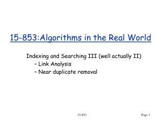
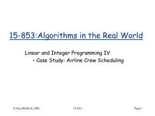
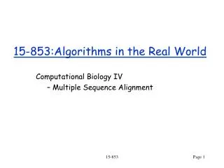
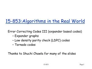
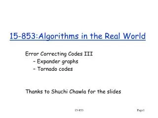
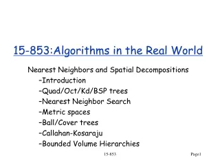
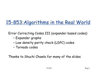
15-853:Algorithms in the Real World. Parallelism: Lecture 1 Nested parallelism Cost model Parallel techniques and algorithms. Andrew Chien, 2008. 16 core processor. 64 core blade servers ($6K) (shared memory). x 4 =. 1024 “ cuda ” cores. Up to 300K servers. Outline.

E N D
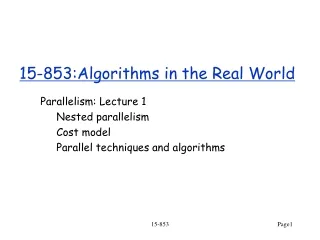
15-853:Algorithms in the Real World Parallelism: Lecture 1 Nested parallelism Cost model Parallel techniques and algorithms 15-853
Andrew Chien, 2008 15-853
16 core processor 15-853
64 core blade servers ($6K)(shared memory) x 4 = 15-853
1024 “cuda” cores 15-853
Up to 300K servers 15-853
Outline • Concurrency vs. Parallelism • Concurrency example • Quicksort example • Nested Parallelism • - fork-join and parallel loops • Cost model: work and span • Techniques: • Using collections: inverted index • Divide-and-conquer: merging, mergesort, kd-trees, matrix multiply, matrix inversion, fft • Contraction : quickselect, list ranking, graph connectivity, suffix arrays 15-853
Parallelism in “Real world” Problems • Optimization • N-body problems • Finite element analysis • Graphics • JPEG/MPEG compression • Sequence alignment • Rijndael encryption • Signal processing • Machine learning • Data mining 15-853
Parallelism vs. Concurrency • Parallelism: using multiple processors/cores running at the same time. Property of the machine • Concurrency: non-determinacy due to interleaving threads. Property of the application. 15-853
Concurrency : Stack Example 1 • struct link {int v; link* next;} • struct stack { link* headPtr; • void push(link* a) { a->next = headPtr; headPtr = a; } • link* pop() { link* h = headPtr; if (headPtr != NULL) headPtr = headPtr->next; return h;}} A H A H 15-853
Concurrency : Stack Example 1 • struct link {int v; link* next;} • struct stack { link* headPtr; • void push(link* a) { a->next = headPtr; headPtr = a; } • link* pop() { link* h = headPtr; if (headPtr != NULL) headPtr = headPtr->next; return h;}} A H B 15-853
Concurrency : Stack Example 1 • struct link {int v; link* next;} • struct stack { link* headPtr; • void push(link* a) { a->next = headPtr; headPtr = a; } • link* pop() { link* h = headPtr; if (headPtr != NULL) headPtr = headPtr->next; return h;}} A H B 15-853
Concurrency : Stack Example 1 • struct link {int v; link* next;} • struct stack { link* headPtr; • void push(link* a) { a->next = headPtr; headPtr = a; } • link* pop() { link* h = headPtr; if (headPtr != NULL) headPtr = headPtr->next; return h;}} A H B 15-853
Concurrency : Stack Example 2 • struct stack { link* headPtr; • void push(link* a) { do { link* h = headPtr; a->next = h; while (!CAS(&headPtr, h, a)); } • link* pop() { do { link* h = headPtr; if (h == NULL) return NULL; link* nxt = h->next; while (!CAS(&headPtr, h, nxt))} return h;}} A H 15-853
Concurrency : Stack Example 2 • struct stack { link* headPtr; • void push(link* a) { do { link* h = headPtr; a->next = h; while (!CAS(&headPtr, h, a)); } • link* pop() { do { link* h = headPtr; if (h == NULL) return NULL; link* nxt = h->next; while (!CAS(&headPtr, h, nxt))} return h;}} A H 15-853
Concurrency : Stack Example 2 • struct stack { link* headPtr; • void push(link* a) { do { link* h = headPtr; a->next = h; while (!CAS(&headPtr, h, a)); } • link* pop() { do { link* h = headPtr; if (h == NULL) return NULL; link* nxt = h->next; while (!CAS(&headPtr, h, nxt))} return h;}} A H B 15-853
Concurrency : Stack Example 2 • struct stack { link* headPtr; • void push(link* a) { do { link* h = headPtr; a->next = h; while (!CAS(&headPtr, h, a)); } • link* pop() { do { link* h = headPtr; if (h == NULL) return NULL; link* nxt = h->next; while (!CAS(&headPtr, h, nxt))} return h;}} A H B 15-853
Concurrency : Stack Example 2’ • P1 : x = s.pop(); y = s.pop(); s.push(x); • P2 : z = s.pop(); Before: A B C After: B C P2: h = headPtr; P2: nxt = h->next; P1: everything P2: CAS(&headPtr,h,nxt) The ABA problem Can be fixed with counter and 2CAS, but… 15-853
Concurrency : Stack Example 3 • struct link {int v; link* next;} • struct stack { link* headPtr; • void push(link* a) { atomic { a->next = headPtr; headPtr = a; }} • link* pop() { atomic { link* h = headPtr; if (headPtr != NULL) headPtr = headPtr->next; return h;}}} 15-853
Concurrency : Stack Example 3’ • void swapTop(stack s) { link* x = s.pop(); link* y = s.pop(); push(x); push(y); • } • Queues are trickier than stacks. 15-853
Nested Parallelism • nested parallelism = • arbitrary nesting of parallel loops + fork-join • Assumes no synchronization among parallel tasks except at joint points. • Deterministic if no race conditions • Advantages: • Good schedulers are known • Easy to understand, debug, and analyze 15-853
Nested Parallelism: parallel loops • cilk_for (i=0; i < n; i++) • B[i] = A[i]+1; • Parallel.ForEach(A, x => x+1); • B = {x + 1 : x in A} • #pragma omp for • for (i=0; i < n; i++) B[i] = A[i] + 1; Cilk Microsoft TPL (C#,F#) Nesl, Parallel Haskell OpenMP 15-853
Nested Parallelism: fork-join • cobegin { • S1; • S2;} • coinvoke(f1,f2) • Parallel.invoke(f1,f2) • #pragma omp sections • { • #pragma omp section • S1; • #pragma omp section • S2; • } Dates back to the 60s. Used in dialects of Algol, Pascal Java fork-join framework Microsoft TPL (C#,F#) OpenMP (C++, C, Fortran, …) 15-853
Nested Parallelism: fork-join spawn S1; S2; sync; (exp1 || exp2) plet x = exp1 y = exp2 in exp3 cilk, cilk+ Various functional languages Various dialects of ML and Lisp 15-853
Serial Parallel DAGs • Dependence graphs of nested parallel computations are series parallel • Two tasks are parallel if not reachable from each other. • A data race occurs if two parallel tasks are involved in a race if they access the same location and at least one is a write. 15-853
Cost Model • Compositional: • Work : total number of operations • costs are added across parallel calls • Span : depth/critical path of the computation • Maximum span is taken across forked calls • Parallelism = Work/Span • Approximately # of processors that can be effectively used. 15-853
Combining costs • Combining for parallel for: • pfor (i=0; i<n; i++) • f(i); work span 15-853
Why Work and Span • Simple measures that give us a good sense of efficiency (work) and scalability (span). • Can schedule in O(W/P + D) time on P processors. • This is within a constant factor of optimal. • Goals in designing an algorithm • Work should be about the same as the sequential running time. When it matches asymptotically we say it is work efficient. • Parallelism (W/D) should be polynomial O(n1/2) is probably good enough 15-853
Example: Quicksort • function quicksort(S) = • if (#S <= 1) then S • else let • a = S[rand(#S)]; • S1 = {e in S | e < a}; • S2 = {e in S | e = a}; • S3 = {e in S | e > a}; • R = {quicksort(v) : v in [S1, S3]}; • in R[0] ++ S2 ++ R[1]; • How much parallelism? Partition Recursive calls 15-853
Quicksort Complexity Sequential Partition and appending Parallel calls Work = O(n log n) partition append (less than, …) Parallelism = O(log n) Span = O(n) Not a very good parallel algorithm *All randomized with high probability 15-853
Quicksort Complexity • Now lets assume the partitioning and appending can be done with: • Work = O(n) • Span = O(log n) • but recursive calls are made sequentially. 15-853
Quicksort Complexity Parallel partition Sequential calls Work = O(n log n) Span = O(n) Parallelism = O(log n) Not a very good parallel algorithm *All randomized with high probability 15-853
Quicksort Complexity • Parallel partition • Parallel calls Span = O(lgn) Work = O(n log n) Parallelism = O(n/log n) Span = O(lg2 n) A good parallel algorithm *All randomized with high probability 15-853
Quicksort Complexity • Caveat: need to show that depth of recursion is O(log n) with high probability 15-853
Parallel selection {e in S | e < a}; S = [2, 1, 4, 0, 3, 1, 5, 7] F = S < 4 = [1, 1, 0, 1, 1, 1, 0, 0] I = addscan(F) = [0, 1, 2, 2, 3, 4, 5, 5] where F R[I] = S = [2, 1, 0, 3, 1] Each element gets sum of previous elements. Seems sequential? 15-853
sum [3, 6, 4, 12] recurse [0, 3, 9, 13] sum [2, 7, 12, 18] interleave [0, 2, 3, 7, 9, 12, 13, 18] Scan [2, 1, 4, 2, 3, 1, 5, 7] [0, 2, 3, 7, 9, 12, 13, 18] 15-853
Scan code function addscan(A) = if (#A <= 1) then [0] else let sums = {A[2*i] + A[2*i+1] : i in [0:#a/2]}; evens = addscan(sums); odds = {evens[i] + A[2*i] : i in [0:#a/2]}; in interleave(evens,odds); W(n) = W(n/2) + O(n) = O(n) D(n) = D(n/2) + O(1) = O(logn) 15-853
Parallel Techniques • Some common themes in “Thinking Parallel” • Working with collections. • map, selection, reduce, scan, collect • Divide-and-conquer • Even more important than sequentially • Merging, matrix multiply, FFT, … • Contraction • Solve single smaller problem • List ranking, graph contraction • Randomization • Symmetry breaking and random sampling 15-853
Working with Collections • reduce [a, b, c, d, … • = a b c d + … • scan ident [a, b, c, d, … • = [ident, a, a b, a b c, … • sort compF A • collect [(2,a), (0,b), (2,c), (3,d), (0,e), (2,f)] • = [(0, [b,e]), (2,[a,c,f]), (3,[d])] 15-853