Systems Concepts

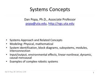
1. Systems Concepts Dan Popa, Ph.D., Associate Professor popa@uta.edu, http://ngs.uta.edu • Systems Approach and Related Concepts • Modeling: Physical, mathematical • System identification, block diagrams, subsystems, modules, interconnection • Input/output, environmental effects, linear-nonlinear, dynamic, causal-noncausal • Examples of complex robotic systems

2. Signals and Systems • Signal: • Any time dependent physical quantity • Electrical, Optical, Mechancal • System: • Object in which input signals interact to produce output signals. • Some have fundamental properties that make it predictable: • Sinusoid in, sinusoid out of same frequency (when transients settle) • Double the amplitude in, double the amplitude out (when initial state conditions are zero)

3. Signal Classification • Continuous Time vs. Discrete Time • Telephone line signals, Neuron synapse potentials • Stock Market, GPS signals • Analog vs. Digital • Radio Frequency (RF) waves, battery power • Computer signals, HDTV images

4. Signal Classification • Deterministic vs. Random • FM Radio Signals • Background Noise Speech Signals • Periodic vs. Aperiodic • Sine wave • Sum of sine waves with non-rational frequency ratio

5. System Classification • Linear vs. Nonlinear • Linear systems have the property of superposition • If U →Y, U1 →Y1, U2 →Y2 then • U1+U2 → Y1+Y2 • A*U →A*Y • Nonlinear systems do not have this property, and the I/O map is represented by a nonlinear mapping. • Examples: Diode, Dry Friction, Robot Arm at High Speeds. • Memoryless vs. Dynamical • A memoryless system is represented by a static (non-time dependent) I/O map: Y=f(U). • Example: Amplifier – Y=A*U, A- amplification factor. • A dynamical system is represented by a time-dependent I/O map, usually a differential equation: • Example: dY/dt=A*u, Integrator with Gain A. Exact Equation, nonlinear Approximation around vertical equilibrium, linear Mandelbrot set, a fractal image, result of a Nonlinear Discrete System Zn+1=Zn²+C

6. System Classification • Time-Invariant vs. Time Varying • Time-invariant system parameters do not change over time. Example: pendulum, low power circuit • Time-varying systems perform differently over time. Example: human body during exercise. • Causal vs. Non-Causal • For a causal system, outputs depend on past inputs but not future inputs.Examples: most engineered and natural systems • A non-causal system, outputs depend on future inputs. Example: computer simulation where we know the inputs a-priori, digital filter with known images or signals. • Stable vs. Unstable • For a stable system the output to bounded inputs is also bounded. Example: pendulum at bottom equilibrium • For an unstable system the ouput diverges to infinity or to values causing permanent damage. Example: short circuit on AC line.

7. System Modeling • Building mathematical models based on observed data, or other insight for the system. • Parametric models (analytical): ODE, PDE • Non-parametric models: graphical models - plots, look-up cause-effect tables • Mental models – Driving a car and using the cause-effect knowledge • Simulation models – Many interconnect subroutines, objects in video game

8. Types of Models • White Box • derived from first principles laws: physical, chemical, biological, economical, etc. • Examples: RLC circuits, MSD mechanical models (electromechanical system models). • Black Box • model is entirely derived from measured data • Example: regression (data fit) • Gray Box – combination of the two

9. White Box Systems: Electrical • Defined by Electro-Magnetic Laws of Physics: Ohm’s Law, Kirchoff’s Laws, Maxwell’s Equations • Example: Resistor, Capacitor, Inductor

10. RLC Circuit as a System

11. White Box Systems: Mechanical

12. White-Box vs. Black-Box Models

13. Grey-Box Models

14. White Box vs Black Box Models Start to understand simple white continuous time models which are linear Eventually deal with grey-box or black-box models in real-life

15. Linear vs. Nonlinear • Why study continuous linear analysis of signals and systems when many systems are nonlinear in practice? • Linear systems have generic, predictable performance. • Nonlinear systems can be approximated and transformed into linear systems. • Some techniques for analysis of nonlinear systems are based on linear methods • If you don’t understand linear dynamical systems you certainly can’t understand nonlinear systems

16. Application Areas for Systems Thinking • Classical circuits & systems (1920s – 1960s) (transfer functions, state-space description of systems). • First engineering applications: military - aerospace 1940’s-1960s • Transitioned from specialized topic to ubiquitous in 1980s with EE applications to: • Electronic circuit design • Signal and image processing • Networks (wired, wireless), imaging, radar, optics. • Control of dynamical systems • Feedback control, prediction/estimation/identification of systems, robotics, micro and nano systems

17. Diagram Representation of Systems Hierarchical Diagram: Organizations Undirected Graph: Networks Flowchart: Procedures, Software

18. System Simulation Software • Matlab Simulink • http://www.mathworks.com/support/2010b/simulink/7.6/demos/sl_env_intro_web.html • National Instruments Labview • http://www.ni.com/gettingstarted/labviewbasics/environment.htm

19. EE-Specific Diagrams • Block Diagram Model: • Helps understand flow of information (signals) through a complex system • Helps visualize I/O dependencies • Equivalent to a set of linear algebraic equations. • Based on a set of primitives: Transfer Function Summer/Difference Pick-off point • Signal Flow Graph (SFG): • Directed Graph alternative U U2 + U1 U1+U2 U U +

20. EE-Specific Diagrams: Signal Flow Graph (SFG – Directed Graph) Multi-loop Control SFG 2-port circuit SFG

21. EE-Specific Diagrams: Block Diagram Simplification Rules

22. EE-Specific Diagrams: Block Diagram Reduction Rules

23. EE-Specific Diagrams: Block Diagram Reduction Rules

24. Robots as Complex Systems G. Bekey definition: an entity that can sense, think and act. Extensions: communicate, imitate, collaborate Classification: manipulators, mobile robots, mobile manipulators. Sense Think Act Robot

25. Research in Multiscale Robotics atNext Gen Systems (NGS) Group Tools and Fundamentals Established Technologies Emerging Technologies Microsystems & MEMS Nanotechnology Biotechnology Robotics Control Systems Manufacturing & Automation Modeling & Simulation Control Theory Algorithms Small-scale Robotics & Manufacturing Assistive Robots Human-like robots Distributed and wireless sensor systems Micromanufacturing Microrobotics Microassembly Micropackaging Sensor & Actuator Arrays NanoManufacturing New applications for robot systems

26. Control System Block Diagram

27. Automatic Control • Control: process of making a system variable converge to a reference value • If r=ref_value=changing - servo (tracking control) • If r=ref_value=constant - regulation (stabilization) • Open loop vs. closed loop (feedback) control + y + y + r Controller K(s) Plant G(s) Controller K(s) Plant G(s) r - Sensor Gain H(s)

28. Brief History of Feedback Control • The key developments in the history of mankind that affected the progress of feedback control were: • 1. The preoccupation of the Greeks and Arabs with keeping accurate track of time. This represents a period from about 300 BC to about 1200 AD. (Primitive period of AC) • 2. The Industrial Revolution in Europe, and its roots that can be traced back into the 1600's. (Primitive period of AC) • 3. The beginning of mass communication and the First and Second World Wars. (1910 to 1945). (Classical Period of AC) • 4. The beginning of the space/computer age in 1957. (Modern Period of AC).

29. Primitive Period of AC Float Valve for tank level regulators Drebbel incubator furnace control (1620) (antiquity)

30. Primitive Period of AC James Watt Fly-Ball Governor For regulating steam engine speed (late 1700’s)

31. Classical Period of AC • Stability Analysis: Maxwell, Routh, Hurwitz, Lyapunov (before 1900). • Electronic Feedback Amplifiers with Gain for long distance communications (Black, 1927) • Stability analysis in frequency domain using Nyquist criterion (1932), Bode Plots (1945). • PID controller (Callender, 1936) – servomechanism control • Root Locus (Evans, 1948) – aircraft control • Most of the advances were done in Frequency Domain.

32. Modern Period of AC • Time domain analysis (state-space) • Bellmann, Kalman: linear systems (1960) • Pontryagin: Nonlinear systems (1960) – IFAC • Optimal controls • H-infinity control (Doyle, Francis, 1980’s) – loop shaping (in frequency domain). • MATLAB (1980’s to present) has implemented math behind most control methods.

33. Feedback Control • Role of feedback: • Reduce sensitivity to system parameters (robustness) • Disturbance rejection • Track desired inputs with reduced steady state errors, overshoot, rise time, settling time (performance) • Systematic approach to analysis and design • Select controller based on desired characteristics • Predict system response to some input • Speed of response (e.g., adjust to workload changes) • Approaches to assessing stability

34. Feedback System Block Diagram • Temperature control system

35. Feedback System Block Diagrams • Automobile Cruise Control

36. Key Transfer Functions Reference + Plant Controller S – Transducer

37. Transient Response Characteristics

38. Effect of pole locations Oscillations (higher-freq) Im(s) Faster Decay Faster Blowup Re(s) (e-at) (eat) Positive feedback Pole at 1/A (unstable) Negative feedback Pole at -1/A (stable)

39. Basic Control Actions: u(t)

40. Summary of Basic Control • Proportional control • Multiply e(t) by a constant • PI control • Multiply e(t) and its integral by separate constants • Avoids bias for step • PD control • Multiply e(t) and its derivative by separate constants • Adjust more rapidly to changes • PID control • Multiply e(t), its derivative and its integral by separate constants • Reduce bias and react quickly

41. Conclusion: Control Systems • Abstraction is the basis for system level thinking. Abstraction requires advanced mathematics, and it is especially required of Electrical and Computer Engineers. • Control Theory contains abstractions and generalizations able to guarantee predictable performance of systems under control. • Negative feedback offers numerous advantages: noise rejection, robustness to plant variations, dynamical tracking performance. • Examples of popular control schemes include Proportional-Integral-Derivative (PID) schemes. • Modern control is primarily based on time-domain analysis of state-equations using matrices. • Control engineers can find jobs in any industry. Control concepts can be applied in any engineering industry.