Download

1 / 48
480 likes | 499 Views
Laymen-friendly introduction to ecological implications of global bifurcations using 2D & 3D population models. Study dynamics of species, interactions, and modeling in ecological scenarios. Discusses Allee effect, stability analysis, predator-prey dynamics, and global bifurcations.

E N D
Ecological implications of global bifurcations For the occasion of the promotion of George van Voorn 17 July 2009, Oldenburg
Overview • Laymen-friendly (hopefully) introduction • 2D Allee-model • 3D Rosenzweig-MacArthur model • 3D Letellier-Aziz-Alaoui model • Discussion
Ecology • Study of dynamics of populations of species • Interactions with other species and physical world • Obvious issues temporal and spatial scale
Modeling • Modeling can help in understanding • Common tool selection: • Ordinary differential equations (ODEs) + Ease in use and analysis, explicit in time − Homogeneous space
Example: Allee • Density-dependency affects population Variables (time-dependent): X(t) = # (= number of) Parameters: β = interspecific growth rate (no explicit nutrient modeling) K = carrying capacity (= maximum sustainable # of carrots) ζ = Allee threshold
Dynamics: Allee • Time dynamics of the model: # Too little carrots extinction Enough carrots growth to carrying capacity Too many carrots decline to carrying capacity
Dynamics: Allee • Asymptotic behaviour: X = K # X = ζ X = 0 Stable equilibria: X = 0, X = K Unstable equilibria: X = ζ
Allee with predator x2 • We add a “predator” x1 x1 = prey population x2 = predator population l = extinction threshold, no fixed value (bifurcation parameter) k = carrying capacity, by default 1 c = conversion ratio, by default 1 m = predator mortality rate, no fixed value (bifurcation parameter) Note: dimensionless
Functional response • Predator-prey interaction Functional response linear x1 = prey population x2 = predator population c = conversion ratio, by default 1
Analysis • Asymptotic behaviour (equilibria) • Stability (local info) Jacobian matrix eigenvalues • Variation of parameter (e.g, l and m) • Switch in asymptotic behaviour = bifurcation point • Numerical package AUTO
Equilibria • 2D Allee model has the following equilibria: E0 = (0,0), stable E1 = (l,0), unstable E2 = (k,0), with k≥l, depends E3 = (m,(m-l)(k-m)), depends
Analysis 2D Allee Two-parameter plot of equilibria depending on m vs l Mortality rate of rabbits Allee threshold for carrots Plot has several regions: different asymptotic behaviour
Analysis Equilibrium: Only prey m > 1 Equilibrium: Predator-prey Transcritical bifurcationTC2: transition to a positive equilibrium
Analysis Predator-prey Equilibrium Predator-prey Cycles Hopf bifurcationH3: transition from equilibrium to stable cycle
Periodic behaviour • Also: limit cycle, oscillations • Hopf bifurcation, also local info # #
Phase plot Orbits starting here go to (0,0) Allee effect Attracting region # Bistability: Depending on initial conditions to E0 or E3/Cycle # l = 0.5, m = 0.74837
Problem… Time-integrated simulations extinction of both species What do we miss? Local info not sufficient Predator-prey Cycles Extinction Prey AND predator !!
Extinction All orbits go to extinction! “Tunnel” # Bistability lost; Allee-threshold gone # l = 0.5, m = 0.735
What happens is … Manifolds of two equilibria connect: Limit cycle “touches” E1/E2 # Heteroclinic orbit connecting saddle point to saddle point # l = 0.5, m = 0.73544235…
New phenomenon • Explains transition to extinction • NOT local info global bifurcation • Heteroclinic connection between two saddle equilibria
Homotopy technique • Need new technique(s): global info • Take an educated guess • Formulate criteria • Convert fault to continuation parameter • Change parameter to match criteria find connection
Method Δx1 = 0 ξ*w ε*v E1 E2 l = 0.5, m = 0.7 (shot in direction unstable eigenvector) l = 0.5, m = 0.7354423495 (connecting orbit)
Global bifurcation in Allee Using developed homotopy method • Regions: • Only prey • Predator –prey • 0. Extinct
Counter-intuitive Bizar: lower mortality rate kills the whole population… • Regions: • Only prey • Predator –prey • 0. Extinct Mortality rate of rabbits 2 Overharvesting or ecological suicide
Add another… • Rosenzweig-MacArthur 3D food chain model, no Allee-effect where (Holling type II) x = variable d = death rate note: dimensionless
Equilibria • There are 4 equilibria:
Chaos • New type of behaviour possible # A-periodic, but still “stable”
Bifurcation diagram Extreme values for top predator are plotted as function of one parameter # d1=0.25 d2
Bifurcation diagram Chaotic Extinct PeriodicStable coexistence # d1=0.25 d2
Global bifurcations Region of extinction marked by global bifurcation # d1=0.25 d2 Saddle limit cycle
New technique • This is a homoclinic cycle-to-cycle connection • No technique thusfar for detection and continuation • Formulation of new criteria • Adaptation of homotopy method
Global bifurcation • Using new technique: # d1=0.25 d2 = 0.0125 # # Connecting orbit from saddle limit cycle to itself
Bifurcation diagram Two parameters 0: no top predator SE: stable existence P: periodic solutions C: Chaos “Eye”: extinction 0 SE d2 P P C d1 Family of tangencies of connecting orbit boundary of chaotic behaviour (boundary crisis)
Different model • Letellier & Aziz-Alaoui (2002)
Different model • Letellier & Aziz-Alaoui (2002) Identical to Rosenzweig-MacArthur Biological interpretation: - No dependence prey density - Different dependence predator density
One-parameter diagram c0 = 0.038 # a1 As compared to RM: two chaotic attractors Two different global bifurcations
One-parameter diagram c0 = 0.038 # a1 First globif bifurcation boundary crisis No stable equilibrium, shift, but… survival
One-parameter diagram c0 = 0.038 # a1 Second global bifurcation interior crisis Change of chaotic attractor
One-parameter diagram Chaos c0 = 0.038 # Low period limit cycle a1 Disappearance of one chaotic attractor Hysteresis (Scheffer) & simplification of system
Discussion • Connection types and ramifications • Allee: heteroclinic point-to-point overharvesting • RM: homoclinic saddle cycle chaos disappears, extinction top predator • L&AA: two homoclinic saddle cycle hysteresis, persistence of top predator
Discussion • Global bifurcations mark different transitions than local • Required development new method • Implemented in AUTO • Essential for analysis • No obvious coupling connection type with biological consequences
Acknowledgements • Bas Kooijman, Bob Kooi • Dirk Stiefs, Ulrike Feudel, Thilo Gross • Yuri Kuznetsov, Eusebius Doedel • Martin Boer, Lia Hemerik • Funding: NWO
George.vanVoorn@wur.nl • www.biometris.wur.nl/ • www.bio.vu.nl/thb/research/project/globif/ Thank you for your attention!
Equilibria • The relevant equilibria now are E0 = (0,0,0) E1 = (1,0,0) E3 = (X1*,X2*,0) No stable equilibrium all 3 species Default parameter values:
Proof: maps # # T+1 T+2 # # T T At the point where chaos disappears we plot the number of bears at time T+n as function of number at time T
Proof: maps # # T+1 T+2 # # T T First globif (upper chaotic attractor) is homoclinic period 1 Second (lower chaotic attractor) homoclinic period 2