Download
1 / 20
200 likes | 299 Views
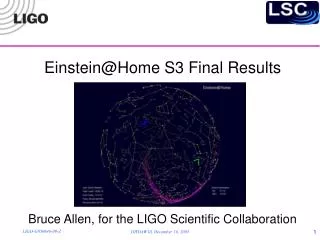
Einstein@Home S3 Final Results Bruce Allen, for the LIGO Scientific Collaboration. Internet. What is Einstein@Home?. Public distributed computing project to look for isolated pulsars in LIGO/GEO data http://einstein.phys.uwm.edu /

E N D
Einstein@Home S3 Final Results Bruce Allen, for the LIGO Scientific Collaboration
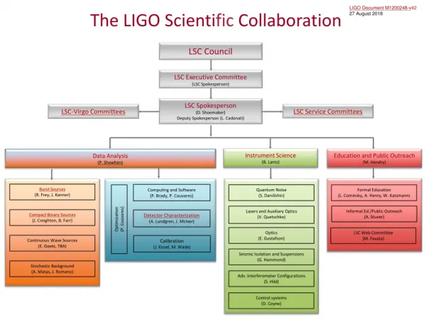
Internet What is Einstein@Home? • Public distributed computing project to look for isolated pulsars in LIGO/GEO data http://einstein.phys.uwm.edu/ • Makes use of the Fstatistic methods (JKS) and code developed over the past few years by the LSC CW search group. • Currently have 142000 users and 240000 computers from 167 countries, delivering ~70 Tflops of CPU, 24 x 7. • Participants go to web page, download BOINC client (Windows, Mac OS X, Linux) and install it. Total time: ~2 minutes. • BOINC client gets frequency-domain data from download server (fraction of Hz) and analyzes it. • Server at UWM, data mirrors at AEI (Berlin), Penn State, MIT, Glasgow.
Goals • The search is for detection, not for setting upper limits. • Intent is to find any isolated pulsars ‘in our backyard’, meaning close enough to generate signals that will show up after coherent integration of ~10 hour data segments. • Use existing documented and tested search methods and code. These methods have been used in the published LIGO S1 and to-be-published LIGO S2 analysis. • Also a wonderful outreach activity to involve the general public in cutting-edge scientific research!
Schematic • Data Preparation • data selection • time-domain calibration • windowing/FFT • injection of software simulated signals SERVER PARTICIPANT’S MACHINE … Search 0.1 Hz Search 0.1 Hz Search 0.1 Hz • Result Postprocessing done on Einstein@Home server
How is the S3 data prepared? • We use the most sensitive 600 hours of LIGO S3 data (from H1). • Data is calibrated in the time domain to make h(t), bandpass filtered and windowed. • 30-minute segments are Fourier Transformed to make Short Fourier Transform (SFT) data sets. • Known (origin identified/understood) instrumental lines are replaced with Gaussian noise random numbers, with amplitude chosen to match at boundaries. • Total data set is 1200 x 30 min SFTs, 50->1500.5Hz. • Data to distribute: 2901 overlapping files of ~14 MB, each containing 1200 SFTs covering ~ 0.7 Hz.
Simulated signals • The data set includes 17 simulated signals: • 11 ‘hardware injections’. These were added into the length control system during the science run. They were ‘turned on’ between 1/3 and 2/3 of the time. • 6 ‘software injections’. These were added (in the frequency domain) into the calibrated SFT data long after the S3 run was over. • These simulated signals are a useful way to gain confidence in the results and to understand the search pipeline.
Search Method • There are a total of 60 ten-hour data segments • Each host machine: • Gets TWO ten-hour segments • Searches each segment with an isotropic sky grid of ~ 31000 points over 0.1 Hz band • Records all points (, , f, F) for which 2F=25 exceeded. Points are clustered by frequency. • To reduce size of data set, keep ONLY those points for which 2F=25 was exceeded in BOTH ten-hour segments of data. Window is 1mHz in f and 0.02 radians in Ω. • Returns resulting set of candidates (, , f, 2 F) to the server • Total number of workunits: 14505 x 30 = 435150 • Host machines are unreliable (overclocking, bad memory, cheating). So each workunit is done by at least three different users, and the results are validated by comparison. • Postprocessing on project server: count number of candidates in cells of 1mHz and 0.02 radians.
What would a pulsar look like? • Final output is 14505 x 30 = 435150 files. Each file covers 0.1 Hz and includes candidates that appeared over threshold in two ten-hour data segments • Post-processing step: find points on the sky and in frequency that exceeded threshold in many of the sixty ten-hour segments Simulated (software) pulsar signal in S3 data
How far away could we see? Sensitivity is as expected based on a ten-hour coherent integration time, with the measured noise curve. The simulated source on the previous page is at ~100 pc. Assumes star ellipticityof =10-6
A typical clean band Results from a clean band (300-325 Hz): no visible sources
A band with instrumental lines S3 band (340-350Hz) containing violin modes
Sky pattern of instrumental lines { • Pulsar (green) far above the plane of the Earth’s orbit or pulsar (yellow) directly behind the Earth’s orbital velocity around the Sun has minimum modulation • Thus instrumental lines mimic sources in the plane defined by blue/green/yellow points above. • Circle r.n=0on celestial sphere is the “minimum frequency modulation circle” EARTH {
Final S3 analysis results • 50-1500 Hz band shows no evidence of strong pulsar signals in sensitive part of the sky, apart from the hardware and software injections. There is nothing “in our backyard”. • Outliers are consistent with instrumental lines. All significant artifacts away from r.n=0 are ruled out by follow-up studies. WITH INJECTIONS WITHOUT INJECTIONS
Typical hardware injection • Typical ‘signal’ artifact away from the r.n=0 circle is the ‘GEO hardware injected pulsar’ at 1125.65 Hz. • LIGO injection was not realistic: only turned on at the end of the S3.
Study of outliers • After removal of all hardware and software injections,there are 67 frequency bands (0.1 Hz wide) where events appear in 10 or more segments of data. • Each one of these frequency bands was studied. • In 59 of these bands, the artifacts lie on the minimum frequency modulation (r.n=0) circle, consistent with instrumental lines. • In the remaining 8 bands (70.1, 152.7, 614.6, 615.4, 839.1, 947, 1032.5, 1432) Hz there are one or more events away from the r.n=0 circle. • A follow-up study of each of these events was done using more sensitive S4 data (identical analysis pipeline: Einstein@Home on S4 data). No signals were found at the same level of significance (appearing in 10 or more segments). • In some cases, the source of these outliers has been identified.
First artifact example • 70.1174-70.1216 Hz (Subsequently identified as coming from VME clock) • While instrumental lines normally appear on the minimum frequency modulation (r.n=0) circle, they can appear elsewhere.
Second artifact example • S3 data • Artifacts off r.n=0 appear to be scatter from set of artifacts on r.n=0. • 615.4214-615.5446 Hz • Unidentified line • S4 data • This artifact does not appear in S4 data at all.
The most significant S3 events • Study of Gaussian noise (from one frequency band used for software injections) shows typical maximum correlation of five data segments. • Highly significant events (25 or more data segments) are all on r.n=0 circle. • Conclusion: no high confidence detections in S3.
Einstein@Home future plans • S4 analysis using identical code and methods finished: under internal review. • For about five months the CW search group has been working to implement an improved search algorithm in Einstein@Home • Near optimal grid (within ~2) on the sky and in frequency and df/dt • Explicit search over spindowns (df/dt) corresponding to pulsars older than a few thousand years. Previous searches had |df/dt|<1/(integration time)2. • Increase coherent integration time from 10 to 30 hours (17 such segments). • Distribute the sky grid with work rather than compute on host machines • Each host machine still does the entire sky, but searches a variable-sized region of frequency df ~ f-3 and only one stretch of data. • Each host machine returns list of ‘top 13,000 events’. • This effectively gives a ‘floating threshold’. In frequency bands free of instrumental artifacts, this increases potential sensitivity. In frequency bands which are corrupted by instrumental lines, it prevents ‘swamping’ of server by too much output. • Required new checkpointing code and routines • Explicit search over spindown required a new validator. Finally working! • Hope to have this up and running on the public project very soon. • Planning a systematic software injection study over large range in frequency. • In the future, Einstein@Home will be the primary large computing resource for the LSC CW search group.