Download
1 / 50
500 likes | 560 Views
Momentum budget of a squall line with trailing stratiform precipitation: Calculations with a high-resolution numerical model. Yang, M.-J., and R. A. Houze , Jr., 1996: Momentum budget of a squall line with trailing stratiform precipitation: Calculations with a

E N D
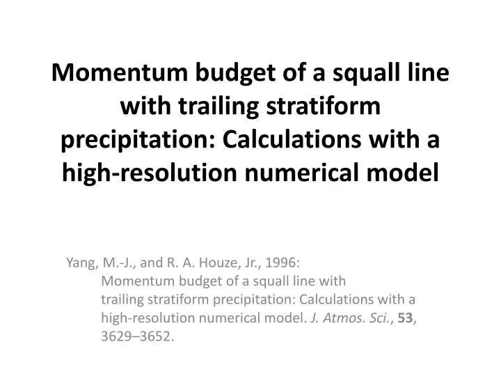
Momentum budget of a squall line with trailing stratiform precipitation: Calculations with a high-resolution numerical model Yang, M.-J., and R. A. Houze, Jr., 1996: Momentum budget of a squall line with trailing stratiform precipitation: Calculations with a high-resolution numerical model. J. Atmos. Sci., 53, 3629–3652.
Outline • Keyword • Introduction • Model description • Simulation results • Evolution of momentum generation and advective processes • Area-average momentum budgets • Impact of momentum flux on mean flow • Large-scale momentum budget • Conclusions • Reference
Keyword • Squall line
Squall line propagation Gust front 2000km Shelf Cloud Cold pool 20-50 km Pictures originated from http://www.crh.noaa.gov/sgf/?n=spotter_squall_lines
Introduction • By MM4 simulation of the 10-11 June 1985 squall line in the Preliminary Regional Experiment for Storm-scale Operational Research Meteorology(PRE-STORM). (Cunning,1986.; Gao et al.,1990) They investigated the meso-β-scale momentum budget and its effects on large-scale mean flow, and found that cross-line momentum generation was the strongest contribution to the momentum budget. • Convectively generated downdrafts were as important as updrafts in vertically transporting horizontal momentum within both the convective and stratiform regions. • Gallus and Johnson(1992) used rawinsonde data to diagnose the momentum fluxes and tendencies in the same squall line case as above. They found a strong midlevel mesolow, which contributed to RTF tendency in the vicinity of a FTR tendency elsewhere through most of the storm.
Introduction • The convective and stratiform precipitation regions are distinct both kinematically (Houze 1982,1989) and microphysically (Houze 1989,1993; Braun and Houze 1994a,b, 1995a,b), and the large-scale flow responds fundamentally differently to the vertical heating profiles in these two regions(Mapes 1993; Mapes and Houze 1995). • The radar echo structure in the convective and stratiform precipitation regions is also distinct, as a result of the different kinematics and microphysics, and techniques are available to separate the convective and stratiform precipitation regions based in their different reflectivity structure (Churchill and Houze 1984; Steiner et al. 1995).
Until now, the separate roles of the convective and stratiform precipitation regions have not been investigated in terms of how they may influence the large-scale horizontal momentum field. • Objective of this study: to investigate the momentum budget of a 2D squall line with leading-line/trailing-stratiform structure and thereby gain insight into contributions of the convective and stratiform precipitation regions to the momentum transports over a large-scale region containing the storm.
Model description • 2-D version of the Klemp and Wilhelmson(1978) compressible nonhydrostatic cloud model, as modified by Wilhelmson and chen(1982). • Microphysical bulk parameterization is described by Lin et al.(1983), with improvements suggested by Potter(1991). • Ice-phase microphysics is included. • Integrated for 15h. (Because of the constant favorable condition, the storm did not actually died before 15h. ) • The basic-state environment is assumed constant in time and horizontally homogeneous. • Coriolis force, surface drag, and radiation effects are neglected. • Outout time interval : 2min.
y(along-line) x(cross-line) z (vertical) No variation, no velocity component. • Grids settings: • Open boundary with phase speed c*=30 m/s • To keep the storm in the fine grid region, the model’s domain translated with the storm. model top : 21.7km Δz=550m x(cross-line) 455 grids, 4814 km Picture originated from ’NOAA radar observation. ’ x(cross-line) ... …. … … … … Stretched mesh 70 grids , 2250km 1.075:1 Fine grid region 315 grids Δx=1 km 62grids y(along-line) Δz=140m Picture originated from,’ Atmospheric Science_University of illinois at urbana-champaign website ‘
Initialization Environment- based on the 2331 UTC 10 June 1985 sounding data at Enid, Oklahoma.(4h before the squall line passed the station.) Convection- triggered by a 5-km deep, 170-km wide cold pool with a -6-K potential temperature and a -4 g/kg water vapor. Picture originated from,’ Yang, M.-J., and R. A. Houze, Jr., 1995: Sensitivity of squall-line rear inflow to ice microphysics and environmental humidity.‘ Fig.5
Three time periods : t=7.5-8.5h (initial stage) t=10-11h (mature stage) t=12.5-13.5h (slowing-decaying stage) • Four subregions : CV (Convective Precipitation) SF (Stratiform Precipitation) RA (Rear Anvil) FA (Forward Anvil) Convective precipitation region- surface rainfall rate ≥ 15 mm/h. or the gradient of rainfall rate > 5 mm/h/km. Stratiform precipitation region- not satisfying these criteria. Fine grid region 315km
Kinematic Fields Shaded cloudy region-time-averaged nonprecipitating hydrometeor(cloud water and cloud ice) mixing ratio ≥ 0.1g/kg Solid line- RTFflow Dashed line- FTR flow Heavy outline-storm precipitation boundary (time-averaged modeled radar reflectivity 15-dBZ contour) • U-c(storm-relative horizontal wind)
Kinematic Fields Solid line- positive Dashed line- negative • ω (vertical celocity)
Thermal Fields • θ' (potential temperature perturbation) Solid line- positive Dashed line- negative
Pressure Fields Solid line- positive Dashed line- negative • p’ (pressure perturbation) L H L L H L L H
Subregional contributions to the large-scale mean horizontal and vertical velocity fields I physical quantity [I] average I over A <I> average I over subregions 300-km-wide large scale area Fractions of A covered by subregions
Mature period: I=ω • Total curve(A) shows a mean updraft. • Maximum at higher level than CV: • Caused by the effect of the • mesoscale updraft/downdraft in the • SF. 7.5km 5.5km All positive. Maximum: 4km 1.5km PBL top Favorable for the convective cells’ development ahead the gust front.
Mature period: I=u-c The large-scale horizontal wind is Mainly determined by SF. Which shows string FTR flow at midlevels and RTF flow at low levels.
The horizontal momentum equation in a coordinate system moving with the squall line (neglect Coriolis force): nondimensional pressure perturbation specific heat at constant p local tendency in the moving coordinate system (TEN) basic-state virtual potential temperature (TRB) subgrid-scale turbulent mixing (PGF) (HAD) (VAD) ground-relative horizontal wind propagation speed storm-relative horizontal wind ‘
Rewrite in time-averaged form: (TEN) (PGF) (HAD) (VAD) (TRB) ADV=HAD+VAD Generally small Where Three time periods : t=7.5-8.5h (initial stage) t=10-11h (mature stage) t=12.5-13.5h (slowing-decaying stage)
t=7.5-8.5h (initial stage) Solid line- RTFflow Heavily shaded-RTF >3 m/s Dashed line- FTR flow Lightly shaded- FTR < -18 m/s • Consistent with the 2 RTF wind • maximum. • The descending RTF flow is in • part a dynamical response to the • latent cooling process. • (Yang and Houze, 1995b) Consistent with the 2 FTR wind maximum.
t=10-11h (mature stage) Solid line- RTFflow Heavily shaded-RTF >3 m/s Dashed line- FTR flow Lightly shaded- FTR < -18 m/s All features intensified/extended. RTF flow penetration. Resulting in weakening the diverging upper level flow. (Consistent with U-c plot.) L drove the ascending FTR flow and transported hydrometeors rearward to form the stratiform precipitation region. L L In CV, ADV(RTF) worked opposite to PGF(FTR). HAD extended and tilted the FTR flow. RTF flow penetration.
t=12.5-13.5h (slowing-decaying stage) Solid line- RTFflow Heavily shaded-RTF >3 m/s Dashed line- FTR flow Lightly shaded- FTR < -18 m/s All features exhibited a more weakly organized but similar to mature stage. L L
Target: To inquire the role of the cloud system in terms of the deviations from the mean flow. Horizontal averaged in large-scale area A (L=300km) (TEN) (TRB) Horizontal averaged form of momentum equation: means average over a subregioni of A. (PGF) (HAD) (VAD) ADV=HAD+VAD Generally small Since the terms are qualitatively similar during three stages, Only mature stage (t=10-11h) is discussed.
t=10-11h (mature stage) Positive-RTFflow Negative-FTR flow • TRB is very small. • VAD and HAD is roughly out • of phase. • In rear region, all terms are • relatively small. • TEN dominates. • Calculation of the correct • momentum tendency in SF is • essential to computing the overall • effect of the storm on large-scale • momentum field. • TEN is a small residual of other • forcing terms. 4 km 2 km 5 km • TEN is RTF at lower level, which is • similar to SF. • Intensify the RTF flow.
t=10-11h (mature stage), the sum of all subregions. Positive-RTFflow Negative-FTR flow 3 km • TEN is similar to SF. • Once the system is mature, • SF dominates the net momentum • tendency of large-scale region A.
Define means and perturbations of a velocity component V (V=u or w) as basic-state density Time-averaged + Deviation and Space-averaged + Deviation Following Priestly(1949) for the decomposite of large-scale heat fluxes in general circulaions, we decompositethe total vertical flux of storm-relative horizontal momentum into three physically distinct parts. transport by standing eddies. (steady-state meso-scale circulation) transport by transient eddies. (temporally fluctuating convective-scale flow) the momentum transport by steady mean flow. (Mean flow in A) are neglected.) and (Note that
t=10-11h (mature stage) + + = Positive-RTFflow Negative-FTR flow • All fluxes contribute to FTR flow. • Above 6.5km, dominates. • Below 6.5km, dominates.
t=10-11h (mature stage) FTR FTR (< 6.5km) FTR (> 6.5km)
t=10-11h (mature stage) , subregion area-averaged 6.5 km 6.5 km Positive-RTFflow Negative-FTR flow Shaded-velocity product < -5 (m/s)^2
t=10-11h (mature stage) , subregions’ contribution • CV contributes to 65-75% Total.
Rewrite time-averaged form in flux form, And combine with anelastic mass continuity equation : (v is horizontal wind.) Applying area-averaged operator : We have
Time- and space- averaged momentum equation : (TEN) Vertical eddy-flux convergence by standing eddies (VEF) Horizontal PGF (PGF) Horizontal mean-flow flux convergence (HMF) Vertical mean-flow flux convergence (VMF) Generally small Vertical convergence effect =VMF+VEF
t=10-11h (mature stage), large-scale time- and subregion- averaged but except for PGF. Positive-RTFflow Negative-FTR flow • In both rears, PGF is weaker. • In CV, PGF is determined. • In SF, PGF in lower level is smaller. 8 km 6.5 km • In lower level, CV FTR dominant; • In upper level, SF RTF dominant. 2 km
t=10-11h (mature stage), large-scale time- and subregion- averaged but except for VEF. Positive-RTFflow Negative-FTR flow • In CV, VEF pattern. • In SF, RTF/FTR in lower/mid level • is both smaller than in CV. 5 km 3.5 km 1.8 km • In RA, VEF associated with • descending rear inflow made the • pattern. • In FA, VEF produced momentum • change in lower level.
t=10-11h (mature stage), large-scale time- and space- averaged. Positive-RTFflow Negative-FTR flow • VEF and VMF contributed TEN. • HMF is similar to HAD. • mid/low level, • VEF contributed TEN; • higher level, • HMF and PGF contributed TEN. VEF HMF+PGF 8 km • Area average: • the sum of all subregions. VEF
+ + = Positive-RTFflow Negative-FTR flow • x • All fluxes contribute to FTR flow. • Above 6.5km, dominates. • Below 6.5km, dominates.
(TEN) (VEF) (VMF) (PGF) (HMF) L (meso-ϒ-low) Small resudual terms (meso-high) H
Caveat : Coriolis force is not included. • Different CV and SF structure may change the vertical profile of terms.
Reference • http://ww2010.atmos.uiuc.edu/(Gl)/guides/mtr/svr/modl/line/squall.rxml Atmospheric Science_University of illinois at urbana-champaign • http://www.crh.noaa.gov/sgf/?n=spotter_squall_lines • Yang, M.-J., and R. A. Houze, Jr., 1995: Sensitivity of squall-line rear inflow to ice microphysics and environmental humidity. Mon. Wea. Rev., 123, 3175–3193. • http://www.theweatherprediction.com/habyhints/150/ • http://encyclopedia2.thefreedictionary.com/squall+line • http://en.wikipedia.org/wiki/Squall_line • Office of the Federal Coordinator for Meteorology (2008). ”Chapter 2 : Definition” • Yang, M.-J., and R. A. Houze, Jr., 1995: Multicell squall line structure as a manifestation of vertically trapped gravity waves. Mon. Wea. Rev., 123, 641–661. • http://blog.sciencenet.cn/u/sanshiphy • http://www.weatherquestions.com/What_is_a_gust_front.htm • Cunning J., B., Cunning, John B., 1986: The Oklahoma-Kansas. Preliminary Regional Experiment for STORM-Central. Bull. Amer. Meteor. Soc., 67, 1478–1486.
Picture originated from ‘Cunning J., B., Cunning, John B., 1986: The Oklahoma-Kansas. Preliminary Regional Experiment for STORM-Central. Bull. Amer. Meteor. Soc., 67, 1478–1486.’
Picture originated from ‘http://www.weatherquestions.com/What_is_a_gust_front.htm’ A gust front is the leading edge of cool air rushing down and out from a thunderstorm. There are two main reasons why the air flows out of some thunderstoms so rapidly. The primary reason is the presence of relatively dry (low humidity) air in the lower atmosphere. This dry air causes some of the rain falling through it to evaporate, which cools the air. Since cool air sinks (just as warm air rises), this causes a down-rush of air that spreads out at the ground. The edge of this rapidly spreading cool pool of air is the gust front. The second reason is that the falling precipitation produces a drag on the air, forcing it downward. If the wind following the gust front is intense and damaging, the windstorm is known as a downburst.
For unsaturated air, , Consider the pressure,
Picture originated from ‘Stratiform precipitation in regions of convection: a meteorology paradox?’ Robert A. Houze Jr., University of Washington, Seatle, Washington