Download
1 / 40
400 likes | 421 Views
MA Activities since PM1. Orbit Selection Update of RC analysis to users needs Investigation of “synodic” sub-cycles Atmospheric Density and Drag Update of models to be ECSS-compliant Assessment of drag levels over a full solar cycle Assessment of differential drag for Cartwheel formation

E N D
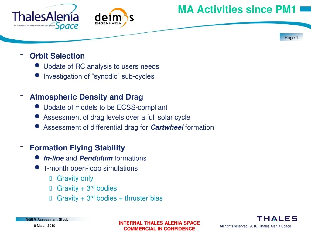
MA Activities since PM1 • Orbit Selection • Update of RC analysis to users needs • Investigation of “synodic” sub-cycles • Atmospheric Density and Drag • Update of models to be ECSS-compliant • Assessment of drag levels over a full solar cycle • Assessment of differential drag for Cartwheel formation • Formation Flying Stability • In-line and Pendulum formations • 1-month open-loop simulations • Gravity only • Gravity + 3rd bodies • Gravity + 3rd bodies + thruster bias
Orbit Selection • Users RC requirements/suggestions: • 2 orbits: SSO, polar or Bender (62.7°) • Long repeat cycles, e.g. 30 and 181 days • Short sub-cycles, e.g. 7 and 12 days • Optional extra sub-cycle: 4 days • General comments: • Sub-cycles are the main altitude drivers • Slight tolerances (e.g. ±1 day) widen the altitude choice,especially accepting odd sub-cycles (e.g. 12 → 13 or 11 days) • Very large RCs imply good altitude control: • 181-d RC ⇒ ~15 km between tracks at Equator • ±1 km ground-track control ⇒ ±50 m altitude control
Orbit Selection • Candidates in the 250km – 550 km altitude range: • Sub-cycle = 7 days • RC ≥ 30 days • SSO: 6 altitudes areas • ~ 310 km • ~ 350 km • ~ 390 km • ~ 430 km • ~ 475 km • ~ 515 km
Orbit Selection • Candidates in the 250km – 550 km altitude range: • Sub-cycle = 7 days + 4 days • RC ≥ 30 days • SSO: 2 altitudes areas • ~ 350 km • ~ 475 km Gap evolution for 15+23/32 (347 km) 4-d sub-cycle 7-d sub-cycle
Orbit Selection • Candidates in the 250km – 550 km altitude range: • Sub-cycle = 7 days • RC ≥ 30 days • Polar: 6 altitudes areas • ~ 295 km • ~ 335 km • ~ 375 km • ~ 420 km • ~ 460 km • ~ 505 km • 4-d additional sub-cycle at: • ~ 335 km • ~ 460 km
Orbit Selection • Candidates in the 250km – 550 km altitude range: • Sub-cycle = 7 days • RC ≥ 30 days • 62.7°: 6 altitudes areas • ~ 250 km • ~ 295 km • ~ 335 km • ~ 380 km • ~ 420 km • ~ 465 km • 4-d additional sub-cycle at: • ~ 295 km • ~ 420 km
Orbit Selection • Candidates in the 250km – 550 km altitude range: • Sub-cycle = 12 days • RC = 181 days • SSO: 4 altitudes areas only • ~ 290 km • ~ 385 km • ~ 435 km • ~ 535 km • No 4-d additional sub-cyclepossible
Orbit Selection • Candidates in the 250km – 550 km altitude range: • Sub-cycle = 12 days ± 1 day • RC = 181 days • SSO: many available altitudes • 4-d additional sub-cycles at: • ~ 340 km • ~ 480 km Gap evolution for 15+132/181 (345 km) 4-d sub-cycle 11-d sub-cycle
Orbit Selection • Candidates in the 250km – 550 km altitude range: • Sub-cycle = 12 days ± 1 day • RC = 181 days • Polar: many available altitudes • 4-d additional sub-cycles at: • ~ 325 km • ~ 470 km Gap evolution for 15+132/181 (332 km) 4-d sub-cycle 11-d sub-cycle
Orbit Selection • Candidates in the 250km – 550 km altitude range: • Sub-cycle = 12 days ± 1 day • RC = 181 days • 62.7°: many available altitudes • 4-d additional sub-cycles at: • ~ 285 km • ~ 430 km Gap evolution for 15+132/181 (289 km) 4-d sub-cycle 11-d sub-cycle
Orbit Selection • Candidates in the 250km – 550 km altitude range: • Summary plot showing available altitudes for: • Various sub-cycles: 7d,12d,12d ±1d and 4d (red dots) • Various inclinations: SSO, Polar, 62.7°
Orbit Selection • Candidates in the 250km – 550 km altitude range: • Summary plot showing available altitudes for: • Various sub-cycles: 7d,12d,12d ±1d and 4d (red dots) • Various inclinations: SSO, Polar, 62.7° • Altitude control margins to avoid RC < 30d resonances
Orbit Selection • Combined Sub-Cycles • Given 2 repeat orbits, with sub-cycles N1 and N2, it is possible to obtain a sub-cycle N3 so that: N3 < N1 and N3 < N2 • Example: • 15+2/15 and 14+13/15 • Both have a 15-d RC and a 8-d sub-cycle • The combination offersa 4-d sub-cycle
Orbit Selection • Combined Sub-Cycles • Given 2 repeat orbits, with sub-cycles N1 and N2, it is possible to obtain a sub-cycle N3 so that: N3 < N1 and N3 < N2 • Example: • 15+2/15 and 14+13/15 • Both have a 15-d RC and a 8-d sub-cycle • The combination offersa 4-d sub-cycle • This is due to the contraryfilling directions within the phasing grid
Orbit Selection • Combined Sub-Cycles • Given 2 repeat orbits, with sub-cycles N1 and N2, it is possible to obtain a sub-cycle N3 so that: N3 < N1 and N3 < N2 • Example with candidate orbits: • 15+13/30 and 15+106/181 • The combination creates a new3-d sub-cycle • This does not work on allpairs of orbits.
Analysis of Atmospheric Drag • General Assumptions • Orbit reference altitudes between 300 and 400 km • Polar orbit (Inclination = 89.99 degrees) • Launch date: 2010 • Lifetime: 1 solar cycle • S/C area-to-mass ratio: 1/500 m²/kg • Drag coefficient: 2.2 • Atmospheric Model = Jacchia-Bowman 2006 (JB-2006) • Atmospheric Activity: • Maximum activity level • Mean activity level
Analysis of Atmospheric Drag • Jacchia-Bowman 2006 atmospheric model • Required by ECSS-E-ST-10-04C (Nov.2008) • Better and more accurate mean total atmospheric density • Valid for altitudes over 120 km • Key novel features: • New formulation of semi-annual density variation in thermosphere • New formulation of solar indices • Indices: • F10.7 : radio energy flux • S10.7: EUV radiation Solar Activity • M10.7: MUV radiation • Ap Geomagnetic Activity • Solar Activity indices values provided by ECSS-E-ST-10-04C (Annex A) • Geomagnetic Activity indices given by NASA-MSFC-MSAFE (Jan. 2010 update)
Analysis of Atmospheric Drag • Density comparison of JB-2006 and MSISE-90 results • Maximum solar/geomagnetic activity conditions • Href = 300 km • Period: full solar cycle • Minimum, average and maximum density per orbit vs. time JB-2006 model MSISE-90 model
Analysis of Atmospheric Drag • Density comparison of JB-2006 and MSISE-90 results • Maximum solar/geomagnetic activity conditions • Href = 300 km • Period: 1orbit • Density profile along one orbit JB-2006 model MSISE-90 model
Analysis of Atmospheric Drag • Parametric Study • Orbit reference altitudes from 300 km to 400 km • Solar/geomagnetic activity level: • Maximum activity (MSAFE 95% and Maximum ECSS values) • Mean activity (MSAFE 50% and Mean ECSS values) • Example case: results of drag evolution with time • Maximum solar/geomagnetic activity conditions • Href = 300 km Maximum Drag per orbit Average Drag per orbit Minimum Drag per orbit
Analysis of Atmospheric Drag • Parametric Study • Orbit reference altitudes from 300 km to 400 km • Solar/geomagnetic activity level: • Maximum activity (MSAFE 95% and Maximum ECSS values) • Mean activity (MSAFE 50% and Mean ECSS values) • Example case: results of drag evolution with time • Maximum solar/geomagnetic activity conditions • Href = 300 km Max. of Maximum Drag per orbit Min. of Minimum Drag per orbit
Analysis of Atmospheric Drag • Parametric Study • Orbit reference altitudes from 300 km to 400 km • Solar/geomagnetic activity level: • Maximum activity (MSAFE 95% and Maximum ECSS values) • Mean activity (MSAFE 50% and Mean ECSS values) • Example case: results of drag evolution with time • Maximum solar/geomagnetic activity conditions • Href = 300 km Max. of Average Drag per orbit Average Drag Min. of Average Drag per orbit
Analysis of Atmospheric Drag • Drag results for maximum solar/geomagnetic conditions
Analysis of Atmospheric Drag • Drag results for mean solar/geomagnetic conditions
Analysis of Atmospheric Drag • Summary • Drag in maximum solar/geomagnetic activity conditions • Drag in mean solar/geomagnetic activity conditions
Analysis of Atmospheric Drag • Drag Analysis of Cartwheel Formation • Orbit assumptions • Href = 350 km • Polar orbit • Mean distance between satellites = 75 km • Design solutions: • Δe and Δω • Δe and ΔM • Solar/geomagnetic activity level assumptions: • Maximum activity (MSAFE 95% and Maximum ECSS values) • Mean activity (MSAFE 50% and Minimum ECSS values) Average Density per Orbit
Analysis of Atmospheric Drag • Drag Analysis of Cartwheel Formation • Orbit assumptions • Href = 350 km • Polar orbit • Mean distance between satellites = 75 km • Design solutions: • Δe and Δω • Δe and ΔM • Solar/geomagnetic activity level assumptions: • Maximum activity (MSAFE 95% and Maximum ECSS values) • Mean activity (MSAFE 50% and Minimum ECSS values) Average Density per Orbit Max. of Average Density per orbit Min. of Average Density per orbit case a) case b)
Analysis of Atmospheric Drag • Drag profile over one orbit (Cartwheel) • Maximum solar/geomagnetic activity • Epoch: maximum value of Average Drag per orbit • Drag range: [1.0 – 2.1] mN • Max. differential drag = 0.05 mN • Mean solar/geomagnetic activity • Epoch: minimum value of Average Drag per orbit • Drag range: [0.06 – 0.17] mN • Max. differential drag = 0.01 mN
Analysis of Stability: In-line 1 year propagation • In-line formation: Earth gravity • Polar orbit (Href = 350 km) • Relative distance = 75 km (ΔM) • Earth gravity: 30x30 • 1 month propagation: • Max. Deviation w.r.t. baseline: ~ 0.2 km 1 month propagation
Analysis of Stability: In-line 1 year propagation • In-line formation: Full gravity • Polar orbit (Href = 350 km) • Relative distance = 75 km (ΔM) • Full gravity: Earth, Sun and Moon • 1 month propagation: • Max. Deviation w.r.t. baseline: ~ 0.2 km 1 month propagation
Analysis of Stability: In-line • In-line formation: Full gravity + Differential Thruster bias • Polar orbit (Href = 350 km) • Relative distance = 75 km (ΔM) • Full gravity: Earth, Sun and Moon • Thruster bias = ± 1e-7 m/s2 • 1 month propagation: • Max. Deviation w.r.t. baseline: ~ 1000 km 1 month propagation
Analysis of Stability: Pendulum Differential RAAN drift • Pendulum with Δi: Earth gravity • Polar orbit (Href = 350 km) • Relative mean distance = 75 km (ΔM, Δi) • Earth gravity: 30x30 • 1 month propagation: • Max. Deviation w.r.t. baseline: ~ 200 km 1 month propagation
Analysis of Stability: Pendulum • Pendulum with Δi: Full gravity • Polar orbit (Href = 350 km) • Relative mean distance = 75 km (ΔM, Δi) • Full gravity: Earth, Sun and Moon • 1 month propagation: • Max. Deviation w.r.t. baseline: ~ 200 km 1 month propagation
Analysis of Stability: Pendulum • Pendulum with Δi: Full gravity + Differential Thruster bias • Polar orbit (Href = 350 km) • Relative mean distance = 75 km (ΔM, Δi) • Full gravity: Earth, Sun and Moon • Thruster bias = ± 1e-7 m/s2 • 1 month propagation: • Max. Deviation w.r.t. baseline: ~ 1000 km 1 month propagation
Analysis of Stability: Pendulum • Pendulum with ΔΩ: Earth gravity • Polar orbit (Href = 350 km) • Relative mean distance = 75 km (ΔM, ΔΩ) • Earth gravity: 30x30 • 1 month propagation: • Max. Deviation w.r.t. baseline: ~ 13 km • Max. Deviation w.r.t. design distances: ~ 0.3 km 1 month propagation
Analysis of Stability: Pendulum • Pendulum with ΔΩ : Full gravity • Polar orbit (Href = 350 km) • Relative mean distance = 75 km (ΔM, ΔΩ) • Full gravity: Earth, Sun and Moon • 1 month propagation: • Max. Deviation w.r.t. baseline: ~ 13 km • Max. Deviation w.r.t. design distances: ~ 0.3 km 1 month propagation
Analysis of Stability: Pendulum • Pendulum with ΔΩ : Full gravity + Differential Thruster bias • Polar orbit (Href = 350 km) • Relative mean distance = 75 km (ΔM, ΔΩ) • Full gravity: Earth, Sun and Moon • Thruster bias = ± 1e-7 m/s2 • 1 month propagation: • Max. Deviation w.r.t. baseline: ~ 1000 km 1 month propagation
Analysis of Stability: Conclusion • Conclusions • 3rd Body perturbations have small impact • Differential thrusterbiasdestabilizes the formation in few days • Pendulum formation is more stable with ΔΩ delta in RAAN
Analysis of Atmospheric Drag • JB-2006 behaviour over poles


![Pass Your ISEB-PM1 Exam with Authentic ISEB-PM1 Dumps [PDF]](https://cdn4.slideserve.com/7887711/slide1-dt.jpg)