Probability Distributions

1. Business Statistics Probability Distributions

2. Random Variables… A random variable is a function or rule that assigns a number to each outcome of an experiment. Alternatively, the value of a random variable is a numerical event. Instead of talking about the coin flipping event as {heads, tails} think of it as “the number of heads when flipping a coin” {1, 0} (numerical events)

3. Two Types of Random Variables… Discrete Random Variable – one that takes on a countable number of values – E.g. values on the roll of dice: 2, 3, 4, …, 12 Continuous Random Variable – one whose values are not discrete, not countable – E.g. time (30.1 minutes? 30.10000001 minutes?) Analogy: Integers are Discrete, while Real Numbers are Continuous

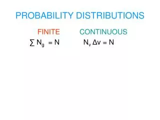
4. Probability Distributions… A probability distribution is a table, formula, or graph that describes the values of a random variable and the probability associated with these values. Since we’re describing a random variable (which can be discrete or continuous) we have two types of probability distributions: – Discrete Probability Distribution and – Continuous Probability Distribution

5. Probability Notation… An upper-case letter will represent the name of the random variable, usually X. Its lower-case counterpart will represent the value of the random variable. The probability that the random variable X will equal x is: P(X = x) or more simply P(x)

6. Discrete Probability Distributions… The probabilities of the values of a discrete random variable may be derived by means of probability tools such as tree diagrams or by applying one of the definitions of probability, so long as these two conditions apply:

7. Example 7.1… Probability distributions can be estimated from relative frequencies. Consider the discrete (countable) number of televisions per household from US survey data… 1,218 ÷ 101,501 = 0.012 e.g. P(X=4) = P(4) = 0.076 = 7.6%

8. Example 7.1… E.g. what is the probability there is at least one television but no more than three in any given household? “at least one television but no more than three” P(1 ≤ X ≤ 3) = P(1) + P(2) + P(3) = .319 + .374 + .191 = .884

9. Example 7.2… Developing a probability distribution… Probability calculation techniques can be used to develop probability distributions, for example, a mutual fund sales person knows that there is 20% chance of closing a sale on each call she makes. What is the probability distribution of the number of sales if she plans to call three customers? Let S denote success, i.e. closing a sale P(S)=.20 Thus SC is not closing a sale, and P(SC)=.80

10. P(S)=.2 P(S)=.2 P(SC)=.8 P(S)=.2 P(S)=.2 P(SC)=.8 P(SC)=.8 P(S)=.2 P(S)=.2 P(SC)=.8 P(SC)=.8 P(S)=.2 P(SC)=.8 P(SC)=.8 Example 7.2… Developing a Probability Distribution… Sales Call 1 Sales Call 2 Sales Call 3 (.2)(.2)(.8)= .032 S S S S S SC S SC S S SC SC SC S S SC S SC SC SC S SC SC SC • X P(x) • .23 = .008 • 3(.032)=.096 • 3(.128)=.384 • 0 .83 = .512 P(X=2) is illustrated here…

11. Population/Probability Distribution… The discrete probability distribution represents a population Example 7.1 the population of number of TVs per household Example 7.2 the population of sales call outcomes Since we have populations, we can describe them by computing various parameters. E.g. the population mean and population variance.

12. Population Mean (Expected Value) The population mean is the weighted average of all of its values. The weights are the probabilities. This parameter is also called the expected value of X and is represented by E(X).

13. Population Variance… The population variance is calculated similarly. It is the weighted average of the squared deviations from the mean. As before, there is a “short-cut” formulation… The standard deviation is the same as before:

14. Example 7.3… Find the mean, variance, and standard deviation for the population of the number of color televisions per household… (from Example 7.1) = 0(.012) + 1(.319) + 2(.374) + 3(.191) + 4(.076) + 5(.028) = 2.084

15. Example 7.3… Find the mean, variance, and standard deviation for the population of the number of color televisions per household… (from Example 7.1) = (0 – 2.084)2(.012) + (1 – 2.084)2(.319)+…+(5 – 2.084)2(.028) = 1.107

16. Example 7.3… Find the mean, variance, and standard deviation for the population of the number of color televisions per household… (from Example 7.1) = 1.052

17. Laws of Expected Value… • E(c) = c The expected value of a constant (c) is just the value of the constant. • E(X + c) = E(X) + c • E(cX) = cE(X) We can “pull” a constant out of the expected value expression (either as part of a sum with a random variable X or as a coefficient of random variable X).

18. Example 7.4… Monthly sales have a mean of $25,000 and a standard deviation of $4,000. Profits are calculated by multiplying sales by 30% and subtracting fixed costs of $6,000. Find the mean monthly profit. 1) Describe the problem statement in algebraic terms: • sales have a mean of $25,000 E(Sales) = 25,000 • profits are calculated by… Profit = .30(Sales) – 6,000

19. Example 7.4… Monthly sales have a mean of $25,000 and a standard deviation of $4,000. Profits are calculated by multiplying sales by 30% and subtracting fixed costs of $6,000. Find the mean monthly profit. E(Profit) =E[.30(Sales) – 6,000] =E[.30(Sales)] – 6,000 [by rule #2] =.30E(Sales) – 6,000 [by rule #3] =.30(25,000) – 6,000 = 1,500 Thus, the mean monthly profit is $1,500

20. Laws of Variance… • V(c) = 0 The variance of a constant (c) is zero. • V(X + c) = V(X) The variance of a random variable and a constant is just the variance of the random variable (per 1 above). • V(cX) = c2V(X) The variance of a random variable and a constant coefficient is the coefficient squared times the variance of the random variable.

21. Example 7.4… Monthly sales have a mean of $25,000 and a standard deviation of $4,000. Profits are calculated by multiplying sales by 30% and subtracting fixed costs of $6,000. Find the standard deviation of monthly profits. 1) Describe the problem statement in algebraic terms: sales have a standard deviation of $4,000  V(Sales) = 4,0002 = 16,000,000 (remember the relationship between standard deviation and variance ) profits are calculated by… Profit = .30(Sales) – 6,000

22. Example 7.4… Monthly sales have a mean of $25,000 and a standard deviation of $4,000. Profits are calculated by multiplying sales by 30% and subtracting fixed costs of $6,000. Find the standard deviation of monthly profits. 2) The variance of profit is = V(Profit) =V[.30(Sales) – 6,000] =V[.30(Sales)] [by rule #2] =(.30)2V(Sales) [by rule #3] =(.30)2(16,000,000) = 1,440,000 Again, standard deviation is the square root of variance, so standard deviation of Profit = (1,440,000)1/2 = $1,200

23. Example 7.4 (summary) Monthly sales have a mean of $25,000 and a standard deviation of $4,000. Profits are calculated by multiplying sales by 30% and subtracting fixed costs of $6,000. Find the mean and standard deviation of monthly profits. The mean monthly profit is $1,500 The standard deviation of monthly profit is $1,200

24. Random Variables • Random Variable (RV): A numeric outcome that results from an experiment • For each element of an experiment’s sample space, the random variable can take on exactly one value • Discrete Random Variable: An RV that can take on only a finite or countably infinite set of outcomes • Continuous Random Variable: An RV that can take on any value along a continuum (but may be reported “discretely” • Random Variables are denoted by upper case letters (Y) • Individual outcomes for RV are denoted by lower case letters (y)

25. Probability Distributions • Probability Distribution: Table, Graph, or Formula that describes values a random variable can take on, and its corresponding probability (discrete RV) or density (continuous RV) • Discrete Probability Distribution: Assigns probabilities (masses) to the individual outcomes • Continuous Probability Distribution: Assigns density at individual points, probability of ranges can be obtained by integrating density function • Discrete Probabilities denoted by: p(y) = P(Y=y) • Continuous Densities denoted by: f(y) • Cumulative Distribution Function: F(y) = P(Y≤y)

26. Discrete Probability Distributions

27. Example – Rolling 2 Dice (Red/Green) Y = Sum of the up faces of the two die. Table gives value of y for all elements in S

28. Rolling 2 Dice – Probability Mass Function & CDF

29. Rolling 2 Dice – Probability Mass Function

30. Rolling 2 Dice – Cumulative Distribution Function

31. Expected Values of Discrete RV’s • Mean (aka Expected Value) – Long-Run average value an RV (or function of RV) will take on • Variance – Average squared deviation between a realization of an RV (or function of RV) and its mean • Standard Deviation – Positive Square Root of Variance (in same units as the data) • Notation: • Mean: E(Y) = m • Variance: V(Y) = s2 • Standard Deviation: s

32. Expected Values of Discrete RV’s

33. Expected Values of Linear Functions of Discrete RVs

34. Example – Rolling 2 Dice

35. Case Study 1.1 • Case of a fruit seller who sells strawberries. Product has a very limited shelf life & is useless unless sold on the day of delivery. 1 Case of strawberries costs $20 and the wholesaler receives $50 for it. Cannot specify the number of cases that will be sold on any day, but analysis of past records produced this information. • What is the optimal stock?

36. Case Study 1.2 An airlines needs to make a decision about its Flight 105. Currently there are 3 seats reserved for last minute customers, but the airlines does not know if anyone will buy them. If they release the seats now, they have to sell them for $250 each. Last minute customers must pay $475 per seat. The company also counts a $150 loss of goodwill for every last minute customer who is turned away. • How much revenue will be generated by releasing all 3 seats now? • What is the company’s expected net revenue (revenue less loss of goodwill) if 3 seats are released now? • What is the company’s expected net revenue if 2 seats are released now? • How many seats should be released to maximize expected revenue?

37. Case Study 1.3 In a lottery the total instant winnings of $34.8 million was available in 70 million $1 tickets, with the ticket prizes ranging from $1 to $1,000. Below are various prizes along with the probability of winning. Compute the expected value & standard deviation of the game.

38. Probability Distributions Probability Distributions Discrete Probability Distributions Continuous Probability Distributions Binomial Uniform Poisson Normal

39. Discrete Probability Distributions • A discrete random variable is a variable that can assume only a countable number of values Many possible outcomes: • number of complaints per day • number of TV’s in a household • number of rings before the phone is answered Only two possible outcomes: • gender: male or female • defective: yes or no Count

40. Continuous Probability Distributions • A continuous random variable is a variable that can assume any value on a continuum (can assume an uncountable number of values) • thickness of an item • time required to complete a task • temperature of a solution • height, in inches • These can potentially take on any value, depending only on the ability to measure accurately. Measure

41. The Binomial Distribution Probability Distributions Discrete Probability Distributions Binomial Poisson

42. The Binomial Distribution • Characteristics of the Binomial Distribution: • A trial has only two possible outcomes – “success” or “failure”, “head” or “tail”, “win” or “lose”, “even” or “odd” • There is a fixed number, n, of identical trials • The trials of the experiment are independent of each other • The probability of a success, p, remains constant from trial to trial • If p represents the probability of a success, then (1-p) = q is the probability of a failure

43. Binomial Experiment • Experiment consists of a series of n identical trials • Each trial can end in one of 2 outcomes: Success or Failure, Head or Tail, Win or Lose, Even or Odd • Trials are independent (outcome of one has no bearing on outcomes of others) • Probability of Success, p, is constant for all trials • Random Variable Y, is the number of Successes in the n trials is said to follow Binomial Distribution with parameters n and p • Y can take on the values y=0,1,…,n • Notation: Y~Bin(n,p)

47. Binomial Distribution Settings • A manufacturing plant labels items as either defective or acceptable • A firm bidding for a contract will either get the contract or not • A marketing research firm receives survey responses of “yes I will buy” or “no I will not” • New job applicants either accept the offer or reject it

48. Counting Rule for Combinations • A combination is an outcome of an experiment where x objects are selected from a group of n objects where: n! =n(n - 1)(n - 2) . . . (2)(1) x! = x(x - 1)(x - 2) . . . (2)(1) 0! = 1 (by definition)

49. Binomial Distribution Formula n ! - x x n P(x) = p q x ! ( - ) ! n x P(x) = probability of x successes in n trials, with probability of success pon each trial x = number of ‘successes’ in sample, (x = 0, 1, 2, ..., n) p = probability of “success” per trial q = probability of “failure” = (1 – p) n = number of trials (sample size) Example: Flip a coin four times, let x = # heads: n = 4 p = 0.5 q = (1 - .5) = .5 x = 0, 1, 2, 3, 4

50. Binomial Distribution • The shape of the binomial distribution depends on the values of p and n n = 5 p = 0.1 P(X) Mean .6 .4 .2 • Here, n = 5 and p = .1 0 X 0 1 2 3 4 5 n = 5 p = 0.5 P(X) .6 .4 • Here, n = 5 and p = .5 .2 X 0 0 1 2 3 4 5