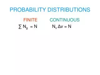
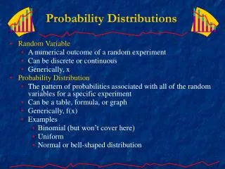
Probability Distributions
Probability Distributions. Mrs. Padilla AP Stats Windsor High School. . Contents The Probability Distribution Elementary Probability Definition of Probability The Binomial Distribution The Mean and Standard Deviation of the Binomial Distribution The Poisson Distribution

Probability Distributions
E N D
Presentation Transcript
ProbabilityDistributions Mrs. Padilla AP Stats Windsor High School
. Contents The Probability Distribution Elementary Probability Definition of Probability The Binomial Distribution The Mean and Standard Deviation of the Binomial Distribution The Poisson Distribution The Normal Distribution Statistical Tales Probability
The Probability Distribution Before discussing the Distribution namely: The Binomial Distribution The Poisson Distribution The Normal Distribution We need first to discuss elementary probability and how to write down probability statements and how to evaluate them. Probability
Elementary Probability • When an ordinary dice is thrown, each of the faces numbered 1, 2 . . . 6 has an equal chance of falling uppermost. There is one chance in six of throwing a 3 so we write the probability statement: Pr(3) or simply P(3) = 1/6 i.e. Pr(not throwing a 3) = 5/6 i.e. Total probability = Pr(3) + Pr(no 3) = 1/6 + 5/6 = 1 Probability
When a fair coin is tossed, it may fall either as a head (H) or as a tail (T) • i.e. We write P(H) = P(T) = 1/2 • If we select a card at random from a pack. • Pr(Ace) = 4/52 = 1/13 • Pr(No Ace) = 48/52 = 12/13 • TPr = Pr(of event happ.) + Pr(event not happ.) • = 4/52 + 48/52 = 1 Probability
Definition of Probability When all the equally possible occurrences have been enumerated, the probability Pr of an event happening is the ratio of the number of ways in which the particular event may occur to the total number of possible occurrences. Probability Statements. Suppose the Pr of a machine producing a defective item is known, then the Pr that in a random sample of eight items produced by the machine, the Pr of not more than 2 being defective will be given by the probability statement: Pr(not more than 2 being defective) = P(≤2) = P(0) + P(1) + P(2) i.e. P(no defects) + P(1 defect) + P(2 defects)
Again the chance or probability of say at least 3 items being defective would be given by: P(≥3) = P(3) + P(4) + . . . + P(8) - - - - (A) Or since the total Pr = 1 we could write (A) as: P(≥3) = 1 – [P(0) + P(1) + P(2)] Note: This is a very useful way of writing (A) and one we will be using regularly in our work. Probability
The Binomial Distribution Before discussing the binomial distribution we need to look at the binomial theorem for a positive integer as a power. (a + b)2 = (a + b)(a + b) = a2 + ab + ba + b2 = a2 +2ab + b2 (a + b)3 = (a + b)(a2 +2ab = b2) = a3 + 3a2b + 3ab2 + b3 This can be extended and the multipliers form Pascal’s triangle as below Each number is the sum of the two numbers above it.
The Binomial Distribution In general the Binomial Expansion of when n is a positive integer is given by: (binomial theorem) Consider the expansion of (¾ + ¼)5 here a = ¾, b = ¼ and n = 5 Exercise Write down the first 3 terms of the Binomial Expansion of (⅞ + ⅛)6 and evaluate their values by the use of a calculator. [ 0.4488, 0.3847, 0.1374]
We can now consider the Binomial Distribution Coin tossing and dice rolling have been used as a means of introducing probability. The consideration of how a coin falls can conveniently illustrate some fundamental probability theory. We must assume that we are dealing with “fair coins” i.e. not two heads or coins that are in any way biased – there is one chance in two or a Pr of 0.5 of obtaining a head and a Pr of 0.5 of obtaining a tail. The development of the Binomial Distribution cab be illustrated by the following simple example of coin tossing. Consider three coins being tossed simultaneously – There are eight possible head (H) and tail (T) combinations:
Tossing three “fair coins” simultaneously • Now consider the probability of obtaining heads when the coins have been tossed. • The probability of obtaining no heads i.e. Pr (no H) is one chance in eight (⅛) i.e. TTT • The probability of obtaining 1 head i.e. Pr (1 H) is three chances in eight (⅜) i.e. TTH, THT, HTT • The probability of obtaining 2 heads i.e. Pr (2 H) is three chances in eight (⅜) i.e. THH, HTH, HHT • Finally the probability of obtaining 3 heads i.e. Pr (3 H) is one chance in eight (⅛) i.e. HHH T T T T TH THT TH H HT T HTH H HT H H H } i.e. We have a) Pr (no H) = ⅛ b) Pr (1 H) = ⅜ c) Pr (2 H) = ⅜ d) Pr (3 H) = ⅛ i.e. Total Probability Pr = 1
Now consider the binomial expansion of (½ + ½) Where (½ + ½) Probability of tailsProbability of heads i.e. Pr of Failurei.e. Pr of Success when the coin is tossed Pr (success) + Pr (failure) = 1 = ⅛ + ⅜ + ⅜ + ⅛ The Pr’s agree with those found above, namely ⅛, ⅜, ⅜ and ⅛ of obtaining no heads, 1 H, 2 H and 3 H respectively when three coins are tossed simultaneously. Probability
We could repeat this for the tossing of four coins. It is clear that with such probability distributions (known as binomial distributions) that the probability results can be obtained by using the binomial distribution. General Binomial Distribution In the binomial distribution of Where p = Pr of the event happening or success q = Pr of the event not happening or failure n = Number of tests Where p + q = 1 Then the terms of the binomial expansion namely: Note the order Give the respective Pr’s of obtaining 0, 1, 2, 3, etc events happening or successes. Probability
Exercises • 1. A Machine produces 20% defective components. In a random sample of 6 components. • Determine the probability that: • There will be 3 defective components • There will be no more than 2 defective components • All the components will be non defective. • The probability of passing an examination is 0.7. Determine the Pr that out of 8 students (a) just 2 (b) more than two will pass the examination. • The incidence of occupational disease in an Industry is such that the workmen have a 25% chance of suffering from it. What is the probability that in a random sample of 7 workmen (a) no one (b) not more than 2 (c) at lease 3 will contract the disease.
1. A Machine produces 20% defective components. In a random sample of 6 components. • Determine the probability that: • There will be 3 defective components • There will be no more than 2 defective components • All the components will be non defective. p = Pr of the event happening or success [0.2] q = Pr of the event not happening or failure [0.8] n = Number of tests [6] Pr (≤2 def) = Pr (0 def) + Pr (1 def) + Pr (2 def) Pr (≤2 def) = 0.26214 + 0.39321 + 0.24576 = 0.9011 = 90.11%
2. The probability of passing an examination is 0.7. Determine the Pr that out of 8 students (a) just 2 (b) more than two will pass the examination. p = Pr of the event happening or success [0.7] q = Pr of the event not happening or failure [0.3] n = Number of tests [8] Pr (>2 pass) = 1 – [Pr (0 pass) + Pr (1 pass) + Pr (2 pass)] Pr (>2 pass) = 1 – [0.00006561 + 0.00122472 + 0.01000188] Pr (>2 pass) = 1 – 0.01129 = 0.98871 = 98.87% Probability
3. The incidence of occupational disease in an Industry is such that the workmen have a 25% chance of suffering from it. What is the probability that in a random sample of 7 workmen (a) no one (b) not more than 2 (c) at lease 3 will contract the disease. p = Pr of the event happening or success [0.25] q = Pr of the event not happening or failure [0.75] n = Number of tests [7] Pr (not 2+ dis) = Pr (0 dis) + Pr (1 dis) + Pr (2 dis) Pr (≤2 inf) = 0.1335 + 0.3115 + 0.3115 = 0.7565 = 75.65% Pr (≥3 inf) = 1 - Pr (≤2 inf) = 1 – 0.7565 = 0.2435 = 24.35% Probability
The Mean and Standard Deviation of the Binomial Distribution The mean or average of a Binomial Distribution λ = n x p The Standard Deviation SD = Distribution about the mean value Example The probability of obtaining a defective resistor is given by 1/10 In a random sample of 9 resistors what is the mean number of defective resistors you would expect and what is the standard deviation? Mean = n x p = 9 x 0.1 = 0.9 SD = √(9x0.1x0.9) = √0.81 = 0.9 Probability
The Poisson Distribution • Under certain conditions the Binomial Distribution assumes a very convenient form. These conditions are: • 1. Sample size is large n ≥ 50 • 2. p = Probability of event occurring is very small p ≤ 0.1 • The mean or average λ is a finite number • λ = n p is ≤ 5 • When these conditions are satisfied, it can be shown • mathematically that the binomial reduces to a convenient • form, where Pr(x) the probability of x successes or events • happening is given by: Where λ is the mean or average value of the distribution. This expression is known as the Poisson Law
Since the Poisson Law has only one constant, namely λ it is easier to tabulate than the Binomial Law which has two independent constants, namely n and p. For the Poisson Law the mean value λ like the Binomial Law is n p i.e. λ = n p Also the Standard Deviation S.D. σ = √(n p q), since q is nearly 1 because p is very small σ = √(n p), = √ (λ) In using the Poisson Law you only have to find one thing, namely the average value λ before you can use it. Note (i) Either you will be told the value of the mean λ in a given question. Or (ii) You can calculate it by using the result λ = n p Probability
Exercises • The number of defective components produced by a machine follows a Poisson Distribution. If the machine produces an average of 3 defective components in a batch of 100, find the probability that in a random batch of 100, (a) 2 (b) more than 2 components will be defective. • p = 0.03 n = 100 λ = n p = 100 x 0.03 = 3 • Now the probability of x defective /100 components is given by Pr(x) in the Poisson Law which states: Probability
No defects • 1 defect • 2 defects • Questions • (a) Pr two defective Pr(2) = 0.2240 = 22.40% • Pr more than 2 Pr(>2) = Pr(3)+Pr(4) + .. + Pr(100) • Pr(>2) = 1 – (Pr(0)+Pr(1)+Pr(2)) • Pr(>2) = 1 – (0.04979+0.14936+0.22404) = 0.5768 = 57.68% • What Binomial Produce? Probability
p = Pr of the event happening or success [0.03] q = Pr of the event not happening or failure [0.97] n = Number of tests [100] Pr (>2 def) = 1 – [Pr (0 pass) + Pr (1 pass) + Pr (2 pass)] Pr (>2 def) = 1 – [0.04755 + 0.14707 + 0.22515] Pr (>2 pass) = 1 – 0.41977 = 0.5802 = 58.02% Probability
Exercises • The Probability of a person having an accident in a certain period of time is 0.001. Determine the probability that out of 2000 people (a) just 3 occur (b) less than 2 people will have an accident. • p = 0.001 n = 2000 λ = n p = 2000 x 0.001 = 2 Probability
No accidents • 1 accident • 2 accidents • 3 accidents • Questions • (a) Pr three accidents Pr(3) = 0.1804 = 18.04% • Pr less than 2 Pr(<2) = Pr(0)+Pr(1) • Pr(<2) = 0.1353 + 0.2707 = 0.4060 = 40.6% Probability
Exercises • The output of an automated machine is inspected by taking samples of 60 items. If the probability of a defective item is 0.0015, find the probability of having (a) two defective items (b) more than two defective items. [0.003701, 0.0001136] • If the probability of suffering a side effect from an injection is 0.002, what is the probability that out of 500 people (a) three, (b) not more than two will suffer a side effect. [0.06131, 0.91970] Probability
The Normal Distribution This was first introduced in 1750 by the mathematician De Moivre, through probability theory. Let us consider a simple example of his work. Suppose we toss 10 coins simultaneously, then the expected probability of obtaining 0, 1, 2, 3, … 10 heads is given by the Binomial Expansion of (½ + ½)10. On expansion we have: Pr(0H) Pr(1H) Pr(2H) etc If we now plot the distribution of the throws of the 10 coins in the form of a frequency polygon, we obtain the diagram on the next slide.
Bell Shaped Curve The distribution is symmetrical about the Mean Value of 5T 5H. If the number of coins were increased to a very large number the distribution approximates to the smooth curve shown on the next slide.
De Moivre called this the Normal Curve Since Head and Tail arrangements are discrete i.e. you cannot have fractional values only whole numbers, like 1H or 2H – you cannot have 2¾H, the curve is not truly continuous. However 50 years later Gauss obtained a truly continuous Normal Curve. Probability
He found that most things in nature gave rise to a Normal Curve or are Normally Distributed e.g. Height of People, Weight of People, Length of Leaves, Weight of Beans, Length around the Forehead, and many others. • Thus a knowledge of the Normal Distribution is very important. • Some important Properties of the Normal Distribution. • The equation of the curve is: • where μ (λ) is the mean, σ is the standard deviation S.D. • Note due to the exponential the curve only touches the x axis at ±∞. You do not need to know this equation.
Area under the Normal Curve • Gauss Showed that the area under the Normal Curve was 1 Unit2. • Since the curve had been obtained through probability theory, where the total probability = 1, there is a connection between probability and the area under the curve. In fact it has been shown that the probability of an event occurring in a Normal Distribution is equivalent to the area a Normal Curve. We will use this in examples later. Probability
~ ~ ~ ~ ~ ~ ~ ~ ~ ~ ~ ~ ~ ~ ~ ~ ~ ~ ~ ~ ~ ~ ~ ~ ~ ~ ~ ~ ~ ~ ~ ~ ~ ~ ~ ~ ~ ~ ~ ~ ~ ~ ~ ~ ~ ~ ~ ~ ~ ~ ~ ~ ~ ~ ~ ~ ~ ~ ~ ~ ~ ~ ~ ~ ~ ~ ~ ~ ~ ~ ~ ~ ~ ~ ~ ~ ~ ~ ~ ~ ~ ~ ~ ~ ~ ~ ~ ~ ~ ~ ~ ~ ~ ~ ~ ~ ~ ~ ~ ~ ~ ~ ~ ~ ~ ~ ~ ~ ~ ~ ~ ~ ~ ~ ~ ~ ~ ~ ~ ~ ~ ~ ~ ~ ~ ~ ~ ~ ~ ~ ~ ~ ~ ~ ~ ~ ~ ~ ~ ~ ~ ~ ~ ~ ~ ~ ~ ~ ~ ~ ~ ~ ~ ~ ~ ~ ~ ~ ~ ~ ~ ~ ~ ~ ~ ~ ~ ~ ~ ~ ~ ~ ~ ~ • Symmetry of the Normal Curve • For a value of plus or minus x away from the mean we have equal areas. Again the areas to the right and left of the mean value µ are equal. Since the Area under the curve is 1 unit2 then the areas are 0.5 each. A A B B -x µ +x Mean Probability
-1σμ +1σ 4. Dispersion or Spread of the Normal Curve The following results are very important (a) The area under the Normal Curve contained between the Mean ± 1 Standard Deviation i.e. μ± 1σ is 68.26% of the area under the whole curve (just over 2/3) • 95% of the area under the curve is contained between μ± 1.96 σ (just under 2) • 99% of the area under the curve is contained between μ± 2.58 σ • After ± 3 σ on either side of the mean, there is hardly any area left 0.0027
STATISTICAL TABLES Area under the Normal Curve For a normal variable x, having a mean μ and a standard deviation σ, the values tabulated give the area under the curve between the mean μ and any multiple of the standard deviation above the mean. The results are given for values of (x – μ)/σ, the Standard Unit Variable (z), at intervals of 0.01. The corresponding areas for deviations below the mean can be found by symmetry. 0 z Probability
Use of the Normal Curve and Normal Probability Tables Suppose a variable is normally distributed about a mean value of 10 with a standard deviation of 0.5. Suppose we want to find the probability of a variable in the distribution having a value between 10.7 and 11.2 To do this we need to find the corresponding area under the normal curve. (As shown) This can be done by standardising the given values of 10.7 and 11.2 – we evaluate each as a Standard Unit Variable z where Probability
When x = 10.7 When x = 11.2 We can now refer to the Table using the values of z of 1.40 and 2.40. The area between 10.7 and 11.2 will be the area up to 11.2 minus the area up to 10.7 Area = z2.40 – z1.40 = 0.4918 – 0.4192 = 0.0726 7.26% of all the variables in this Normal Distribution lie between x = 10.7 and x = 11.2 Probability
Since all the probability questions in a Normal Distribution are equivalent to areas under the Normal Curve (which can be obtained from the table) let us now look at a few examples in evaluating areas under the Normal Curve. Example 1. Find the area under the normal curve between z = -1.36 and z = 0.85 or z-1.36 and z0.85 Putting in the Normal Curve gives us: Area A 0 -1.36 A = 0.4131 Area B 0 +0.85 B = 0.3023 Total Area = 0.7154 A B
Example 2. Find the area between z-2.14 and z-0.93 Area A -2.14 -0.93 A-2.14 = 0.4838 A-0.93 = 0.3238 Area = A-2.14 – A-0.93 Total Area = 0.1600 • What are the areas below the Normal Curve? • Between z1.04 and z2.36 [0.1401] • Between z-0.31 and z1.52 [0.5574] • Area to the left of z-1.42 [0.0778]
Practical Problems on the Normal Distribution 1. The mean of the mass of a set of components is 151Kg and the standard deviation is 15Kg. Assuming that the masses are normally distributed about the mean, find the probability of a single component having a mass of (a) between 120 and 155Kg and (b) greater than 186Kg. (a) μ = 151Kg and σ = 15Kg – we need to calculate z for each value at the extremes of the range. When x = 120Kg z1 = (120 – 151)/15 = -2.07 When x = 155Kg z2 = (155 – 151)/15 = 0.27 Probability
Pr mass between 120Kg and 155Kg is the sum of the areas to the left and the right of the centre. Area = 0.4808 + 0.1064 Area = Pr = 0.5872 (b) To find Pr mass >185Kg z = (185 – 151)/15 = 2.27 Pr of having a mass >185 is the shaded area. This is 0.5 – z2.27 Area = 0.5 – 0.4884 Area = 0.0116 Probability
Practical Problems on the Normal Distribution • The lengths of rods held in stock have a mean of 4.5 m with a standard deviation of 0.05. The distribution of lengths is normal. If the total stock is 1000 rods, how many of the rods can be expected to have (a) a length between 4.5 and 4.6 m and (b) a length less than 4.4 m? • Note The number of rods = Pr x total number of rods. • (a) μ = 4.5 m and σ = 0.05 m – we need to calculate z for each value at the extremes of the range. • When x = 4.5 m z1 = (4.5 – 4.5)/0.05 = 0.00 • When x = 4.6 m z2 = (4.6 – 4.5)/0.05 = 2.00 • The probability of the rod length being between 4.5 and 4.6 m is shown in the diagram on the next slide.
Pr = Area = 0.477.2 Number of rods equals 0.4772 x 1000 = 477 rods • To find the number of rods < 4.4 m • z = (4.4 – 4.5)/0.05 = -2.00 Pr of having a length < 4.4 is the shaded area. This is 0.5 – z-2.00 Area = 0.5 – 0.4772 Area = 0.0228 = 23 rods
Examples • The mean braking load of a sample of concrete blocks was found to be 600N with a standard deviation of 45N. If the loads are normally distributed, calculate the Pr that another block would have a braking load of • (a) between 585 and 610 N [0.2164] • (b) less than 540N [0.0918] • 2. The mean percentage moisture content of a series of 500 test samples of a particular cement mix after a certain time was found to be 27.5% with a standard deviation of 0.5%. Assuming the distribution is normal, find how many of the test samples have a moisture content below 27.1% [106] Probability

